


Abstract
MicroRNAs (miRNAs) are a family of non-coding RNA molecules with vital roles in regulating gene expression. Although researchers have recognized the importance of miRNAs in the development of human diseases, it is very resource-consuming to use experimental methods for identifying which dysregulated miRNA is associated with a specific disease. To reduce the cost of human effort, a growing body of studies has leveraged computational methods for predicting the potential miRNA–disease associations. However, the extant computational methods usually ignore the crucial mediating role of genes and suffer from the data sparsity problem. To address this limitation, we introduce the multi-task learning technique and develop a new model called MTLMDA (Multi-Task Learning model for predicting potential MicroRNA-Disease Associations). Different from existing models that only learn from the miRNA–disease network, our MTLMDA model exploits both miRNA–disease and gene–disease networks for improving the identification of miRNA–disease associations. To evaluate model performance, we compare our model with competitive baselines on a real-world dataset of experimentally supported miRNA–disease associations. Empirical results show that our model performs best using various performance metrics. We also examine the effectiveness of model components via ablation study and further showcase the predictive power of our model for six types of common cancers. The data and source code are available from https://github.com/qwslle/MTLMDA.
INTRODUCTION
MicroRNAs (miRNAs) are a family of non-coding RNA molecules in animal species [1]. The first miRNA (called lin-4) with a molecule of |$22$| ribonucleotides long was discovered in |$1993$| [2]. Although miRNAs are tiny, they play a huge role in biological processes by regulating different genes. These tiny molecules are 21–25 nucleotides in length and are negative regulators of gene expression. At present, a large body of scientific data has confirmed the significance of this tiny molecule in animal cell death and proliferation, hematopoiesis and nervous system patterns [3, 4]. Therefore, abnormal expression of human miRNAs may lead to various serious diseases.
The nature of cancer pathogenesis is the result of genomic dysfunction, and the molecular characterization of miRNAs in different malignancies suggests that they are not only actively involved in the pathogenesis of human cancers, but also play an important role in the recovery process of patients [5]. Furthermore, according to statistics, there are about 200 miRNAs to be significantly dysregulated in various cancer malignancies [6]. For example, vitro experiments found that the down-regulation of let-7 family in humans can up-regulate Rat sarcoma (RAS) proteins, thus leading to lung cancer. Among the differential expression of miRNAs, for breast cancer, miR-10b, miR-125b, and miR-145 were down-regulated while miR-21 and miR-155 were up-regulated, suggesting that they may function as tumor suppressor genes or oncogenes [7, 8]. Overall, the above malignant diseases are mainly formed under the regulation of miRNAs through corresponding genes.
It is well known that Coronavirus disease 2019 (COVID-19) is a contagious disease caused by a type of viruses, which quickly spreads worldwide and results in the COVID-19 pandemic. Up to date, its infection is considered as one of the leading causes of human death. In addition to vaccines already on the market, miRNAs may also be promising options against the new virus. miRNAs can inhibit viral translation after miRNAs attach to the 3-UTR of the viral genome and can also target receptors, structural or nonstructural proteins of severe acute respiratory syndrome coronavirus 2 without affecting human gene expression [9]. MiR-618 is reported to be expressed 1.62 times higher in COVID-19 patients than in healthy people, and it is associated with down-regulation of the immune system [10]. Therefore, miR-618 could be a promising target for the treatment of COVID-19 patients. That is to say, a deep understanding of the potential relationship between miRNAs and diseases is of great significance to human life and health.
Traditional wet experimental methods such as PCR [11], microarray profiling [12] and northern blotting [13] require a lot of time and economic costs in the process of exploring and understanding miRNAs. Besides, benefiting from the rapid development of computer technology, during the gradual establishment and continuous improvement of a large number of relevant bioinformatics databases, the use of computational methods to explore the relationship between miRNAs and diseases has become an essential technical means.
Towards this line of research, over the past few decades, many computational methods have been proposed to investigate the miRNA–disease relationship. Overall, existing research on predicting the relationship between relevant miRNAs and diseases can be mainly divided into two categories: network-based methods and machine learning (ML)-based methods. For Network-based methods, disease similarity, miRNA similarity and miRNA–disease association usually are used to predict potential relationships between diseases and miRNAs [14–17]. For ML-based methods, researchers utilize different ML methods to construct prediction models for the identification of potential miRNA–disease associations[18–21].
However, existing solutions to predict the miRNA–disease relationship still suffer from the following two challenges: (1) Despite the continuous progress of science and technology, the relationship between miRNAs and diseases that have been discovered is still infancy and sparse, which might be insufficient to train an accurate model. (2) Disease–disease similarity and miRNA-miRNA similarity are the key component in most miRNA–disease association prediction models. However, predictive models based on these similarities are not robust enough, and only directly calculating the similarity between miRNAs and diseases fails to capture deep interaction patterns between miRNAs and diseases.
To tackle the above two challenges, in this paper, we propose a novel approach to examine the connections between miRNAs and diseases by introducing the concept of multi-task learning. We have developed a multi-task learning framework that utilizes the relationships between miRNA–disease pairs to construct a disease-gene network. It is worth noting that the two tasks are not independent of each other, but instead are highly correlated due to their shared disease nodes. Consequently, disease nodes are more likely to have a similar proximity structure in the two networks, and to share similar features in non-task-specific latent feature spaces [22]. By leveraging the knowledge contained in different tasks and sharing it with each other, our approach effectively improves the generalization performance of all tasks while also mitigating the issue of data sparsity [23]. The contributions of our work can be summarized in three aspects.
- i.
We propose an effective Multi-Task Learning for Predicting potential miRNA–disease Associations (MTLMDA), which is an end-to-end trainable graph neural network model using GCN-based autoencoder and linear decoder. In the MTLMDA, two sub-networks are constructed by miRNA–disease and gene–disease and are bridged by specially designed cross&compress units. The whole network uses the information learned in the gene–disease sub-network to assist the sub-network of miRNA–disease.
- ii.
To the best of our knowledge, this is the first work to simultaneously consider miRNAs, Genes and diseases in a multi-task learning framework. Through the auxiliary information of the relationship between genes and diseases, we can dig out more relevant information, which can help obtain a more in-depth understanding on the relationships between miRNA and diseases.
- iii.
We verify the effectiveness of our approach via experiments on HMDD v2.0 and HMDD V3.2 dataset. Experimental results demonstrate that our model performs better than state-of-the-art approaches, i.e. our model can predict the miRNA–disease relationship effectively and accurately.
RELATED WORK
Our study is mainly related with the following two topics: network-based methods and machine learning-based methods to predict the relationship between miRNAs and diseases.
Network-based methods
In network-based methods, the computation of various similarities is a key component. Most network-based methods are based on the hypothesis that miRNAs with similar functions are more likely to be associated with similar diseases and vice versa. The hypothesis was first confirmed by Lu et al. [14] through their designed experiments. The research established a theoretical basis for the study of miRNA–disease associations. Moreover, Gu et al. [15] proposed a computational approach to infer disease-related miRNAs based on the theory, and predict miRNA–disease associations in all diseases but does not require negative samples. Chen et al. [24] adopted a global network similarity measure which was different from traditional local network similarity measures and developed an algorithm using random walks with restart to identify miRNA–disease associations. However, it ignores disease phenotypic similarity information, and does not work well when there is no connections between miRNAs and diseases. Xuan et al. [16] addressed the shortcomings of those methods that did not consider the prior information of the local topology of nodes in their network, and built a miRNA network based on the functional similarity of miRNAs.
For disease nodes with known related miRNAs, it can be divided into two types: labeled (i.e. having an association) and unlabeled (i.e. having no association or unknown relationship). Disease similarities were obtained by extending the walk on the miRNA–disease bipartite network for those unlabeled links. The prediction process was then modeled as a random walk on the miRNA network from miRNA-related diseases. For example, Chen et al. [25] developed a model to predict potential miRNAs associated with various complex diseases, named WBSMDA. By integrating disease and miRNA similarities, WBSMDA can be applied to diseases without any known associated miRNAs. However, Wang et al. [26] pointed out that prediction results based on model similarity was not robust enough. Li et al. [27] proposed a label propagation model with linear neighborhood similarity for undiscovered disease-miRNA association prediction by transforming the disease and miRNA similarity into linear domain similarity. Known miRNA–disease associations were used as input for linear propagation, and miRNA–disease associations were scored. Compared with previous models, Chen et al. [17] proposed a new model (i.e. IMCMDA), which used the known associations and the integrated miRNA and disease similarity to discover potential disease-related miRNAs based on matrix completion with network regularization. Wang et al. [28] further developed an effective computational model, named HFHLMDA, that used high-dimensional features and hypergraph learning to predict the relationship between miRNA and disease. Then, Ha et al. [29] further developed an effective computational model, named NCMD, which used node2vec-based neural collaborative filtering for predicting miRNA–disease associations.
With the advancement of network-based methods, Alaimo [30] first proposed a method called ncPred based on a triple network to infer novel ncrna-disease combinations. And later, Yu et al. [31] proposed a three-layer heterogeneous network combined with unbalanced random walk to predict miRNA–disease associations. This method combined lncRNAs, miRNAs and diseases into a heterogeneous network, and leveraged lncRNA as transition information to predict the potential relationship between miRNA and diseases. However, network-based methods ignore the rich structural information contained in the network and cannot fully represent the deep relationships in the miRNA–disease network.
Machine learning-based methods
Machine learning are also widely used in the prediction of miRNA and disease associations. Among those studies, Xu et al. [18] first proposed to rank prostate cancer miRNAs by training the support vector machine (SVM). Chen et al. [32] proposed a model that could not only predict potential miRNA–diseases but also infer the types of miRNA–disease combinations. However, this approach is only suitable for inference of diseases with known miRNA–disease association information. Therefore, Chen et al. [19] developed a random forest-based computational model (i.e. RFMDA) to predict miRNA–disease associations, which could predict unknown miRNA–disease associations through the score labels obtained after implementing random forests. Inspired by the RFMDA model, Yao et al. [33] proposed an improved random forest model to predict potential miRNA–disease combinations. Feature selection through random forest variable importance score can reduce noise information to a greater extent to improve the predictive power of the model. Subsequently, Zheng et al. [34] proposed a new model (MLMDA) to predict miRNA–disease combinations, which further extracted the integrated features through the deep auto-encoder neural network, and finally used the random forest classifier to make predictions. Ji et al. [35] proposed a deep autoencoder model based on the deep learning algorithm, which learned potential miRNA–disease associations from known relation between miRNAs and diseases with an end-to-end manner. Furthermore, Liu et al. [36] developed a framework called SMALF for miRNA and disease association prediction. SMALF used the stacked autoencoder to integrate the node features of the network, and then sent it to XGBoost for miRNA–disease prediction.
Recently, in view of the great capability of learning high-order relationships, some work also adopts graph representation learning to capture the relationship between miRNAs and diseases. For example, Li et al. [20] proposed a graph convolutional network model (i.e. NIMCGCN). However, the performance of NIMCGCN may be limited by the insufficient number of feature representation learning methods. Inspired by the significant promotion of the GraphSAGE algorithm proposed by Hamilton et al. [37], Li et al. [38] proposed a novel graph auto-encoder model, GAEMDA, which gully leveraged the algorithm of GraphSAGE to fully aggregate the miRNA–disease heterogeneous graph information in an end-to-end manner. Wang et al. [39] proposed the NMCMDA model based on the graph neural network. The NMCMDA adopted the graph convolutional autoencoder to calculate the miRNA and disease latent feature representations, and then to predict multiple-category miRNA–disease associations.
A recent study proposed a novel approach called PDMDA (predicting deep-level miRNA–disease associations with graph neural networks and sequence features), which was proposed by Yan et al. [21]. PDMDA use GNN to extract disease feature representation from disease-gene association and PPI network. But, it is still possible to improve the overall prediction performance by considering some biological information. What’s more, Lou et al. [40] proposes a new prediction method named MINIMDA, which learns the embedding representation of miRNA and disease from a multimodal networks which are integrating multiple biological information and then to predict the relationship between miRNA and disease.
However, the aforementioned prediction models for miRNA and disease associations mainly regard the similarity as an important component and do not fully consider the sparsity of identified miRNA–disease relationships, which might lead to inaccurate predictions. In this view, we design a multi-tasking learning model (i.e. MTLMDA) to effectively predict the potential relationship between miRNAs and diseases.
MATERIALS AND METHODS
In this section, we mainly introduce the preparation work required to construct the MTLMDA model as well as the overall framework of the model. In order to improve the readability of the following content, Table 1 summarizes the main notations used in our study.
Summary of main notations
| Variable | Description |
|---|---|
| |$MD$| | miRNA–disease relationship matrix |
| |$n_{d}$| | Number of disease nodes in the HMDD V2.0 -383 |
| |$n_{m}$| | Number of miRNA nodes in the HMDD V2.0 -495 |
| |$GD$| | Gene–disease relationship matrix |
| |$n_{g}$| | Number of gene nodes in the MTLMDA-4395 |
| |$K_{GIP,m}$| | MiRNA Gaussian similarity matrix |
| |$K_{GIP,d}$| | Disease Gaussian similarity matrix |
| |$Y_{m_{i}}$| | The binary row vector in matrix MD |
| |$Y_{d_{i}}$| | The binary column vector in matrix MD |
| |$r_{m},r_{d}$| | The bandwidth of the kernel |
| |$M(i)$| | The |$i$|-th miRNA node feature representation |
| |$D_{1}(\,j)$| | The |$j$|-th disease node feature representation |
| |$G(i)$| | The |$i$|-th gene node feature representation |
| |$D_{2}(\,j)$| | The |$j$|-th diseasenode feature representation |
| |$H_{m}(i),H_{d1}(i)$| | Projection features of miRNA and disease node |
| |$H_{g}(i),H_{d2}(i)$| | Projection features of gene and disease node |
| |$W$| | Different weight matrices |
| |$H_{aux-m},H_{aux-d1}$| | Gene–disease network’s auxiliary information |
| |$H_{aux-g},H_{aux-d2}$| | Mirna–disease network’s auxiliary information |
| |$H_{M}$| | Integrated feature representation of miRNA nodes |
| |$H_{D1}$| | Disease’s integrated representation in miRNA–disease network |
| |$H_{G}$| | Integrated feature representation of gene nodes |
| |$H_{D2}$| | Disease’s integrated representation in gene–disease network |
| |$F_{m}$| | MiRNA node’s final representation in miRNA–disease network |
| |$F_{d1}$| | Disease node’s final representation in miRNA–disease network |
| |$F_{g}$| | Gene node’s final representation in gene–disease network |
| |$F_{d2}$| | Disease node’s final representation in gene–disease network |
| |$\hat{y}_{md}$| | Predicted association probability of miRNA and disease nodes |
| |$\hat{y}_{gd}$| | Predicted association probability of gene and disease nodes |
| |$LOSS{m-d}$| | The loss in the miRNA–disease sub-network |
| |$LOSS{g-d}$| | The loss in the gene–disease sub-network |
| |$LOSS$| | The loss of the entire model |
The construction of subnetworks
In this part, we firstly describe the formation process of the two sub-networks of miRNA–disease and gene–disease, and secondly we depict the way of constructing the Gaussian similarity of the sub-networks.
Human miRNA-disease associations
In our study, miRNA–disease associations is derived from the HMDD v2.0 [41] (https://www.cuilab.cn/hmdd.), which is a mature dataset and contains experimentally verified associations of |$n_{d}(383)$| diseases and |$n_{m}(495)$| miRNAs. The |$5430$| associations of miRNA–disease have been confirmed on this dataset. In the experiments, the identified relationship between diseases and miRNAs is represented as a matrix |$MD$| with |$n_{d}$| columns and |$n_{m}$| rows. The value of an entry is |$1$| if the corresponding disease is associated with the corresponding miRNA, otherwise |$0$| (meaning the relationship is unknown). The matrix |$MD$| is represented as follows:
In total, there are |$189 585$| combinations in |$\mathbf{MD}$| with |$n_{m}(495)$| rows and |$n_{d}(383)$| columns. Besides, |$m_{i}$| represents the |$i$|-th miRNA (also the |$i$|-th row in |$\mathbf{MD}$|), while |$d_{j}$| represents the |$j$|-th disease (the |$j$|-th column in |$\mathbf{MD}$|).
Human genes-disease associations
In our study, the data of gene–disease associations is generated by our manual filtering. Firstly, the original gene–disease relationships are from the DisGeNet [42] (http://www.disgenet.org/home/), which is a database of gene–disease associations. The file named “Curated gene–disease associations” in this database can be downloaded directly from the website and contains |$84 038$| confirmed relationships between human diseases and genes. Then, we select the same disease and related genes as the corresponding miRNA–disease sub-network to form the genes–disease sub-network. Finally, the genes–disease sub-network contains |$9286$| associations between |$n_{d}(383)$| diseases and |$n_{g}(4395)$| genes. Thus, similar to miRNA–disease sub-network, we create a matrix |$\mathbf{GD}$| with |$n_{g}$| rows and |$n_{d}$| columns. If the disease is associated with a gene, the corresponding entry value is |$1$|, |$0$| otherwise. Similarly, the known |$9286$| associations of genes and diseases are used as the positive samples of genes–disease sub-network, and then the negative samples were select from the entries with value |$0$| 0 in |$\mathbf{GD}$|, randomly. The matrix |$\mathbf{GD}$| is represented as follows:
where |$g_{i}$| represents the |$i$|-th gene (|$i$|-th row in |$\mathbf{GD}$|), and |$d_{j}$| represents the |$j$|-th disease, i.e. |$j$|-th column in |$\mathbf{GD}$|.
Gaussian interaction profile kernel similarity for miRNAs and diseases in miRNA–disease subnetwork
Previous studies [43] pointed that similar diseases are often associated with functionally similar miRNAs, based on this hypothesis, Gaussian interaction profile kernel similarity can be well used to simulate the similarity between miRNAs and diseases in miRNA–disease sub-network, and thus is adopted in our study. Specifically, Gaussian interaction profile kernel similarity for miRNAs is calculated by the information of known miRNA–disease associations. Each row in the matrix |$MD$| is represented by a binary vector |$Y_{m}$| that shows the associations between a certain miRNA and various diseases in the miRNA–disease sub-network. The Gaussian interaction profile kernel similarity between miRNA |$m_{i}$| and |$m_{j}$| can be defined as follows:
where |$r_{m}$| represents the bandwidth of the kernel, which can be calculated by:
where |$n_{m}$| represents the total number of miRNAs (|$495$| in this study) and |$r^{\prime}_{m}$| denotes a normalization constant and following previous studies [44], we also set it to be |$1$|. Figure 1 illustrates the Gaussian similarity of some miRNAs in the miRNA–disease sub-network, which represents the potential miRNA–miRNA correlation coefficient in the miRNA–disease sub-network ranging from |$0$| to |$1$|.
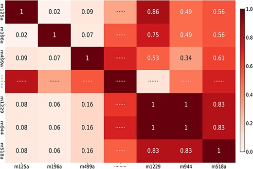
miRNAs Gaussian similarity in miRNA–disease sub-network (Note: ‘m125a,’ ‘m196a,’ ‘m499a,’ ‘m1229,’ ‘m944’ and ‘m518a’ represent miRNA ‘hsa-mir-125a,’ ‘hsa-mir-196a,’ ‘hsa-mir-499a,’ ‘hsa-mir-1229,’ ’hsa-mir-944’ and ‘hsa-mir-518a’, respectively).

Similarly, we can obtain the Gaussian interaction profile kernel similarity of the diseases according to the following formula:
where |$Y_{d}$| is the binary column vector of the matrix |$MD$|, representing associations between miRNAs and each disease; |$n_{d}$| represents the total number of diseases (i.e. |$383$|) and the normalization constant, |$r^{\prime}_{d}$|, is set to |$1$|. Figure 2 visualizes the Gaussian similarity of diseases in the corresponding miRNA–disease sub-network, which represents the potential disease–disease correlation coefficient ranging from |$0$| to |$1$|.
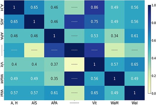
Diseases Gaussian similarity in miRNA–disease sub-network (Note: ‘A,H,’ ‘AIS,’ ‘APA,’ ‘Vit,’ ‘WaM’ and ‘WaI’ represent diseases ‘Abortion, Habitual,’ ‘Acquired Immunodeficiency Syndrome,’ ‘ACTH-Secreting Pituitary Adenoma,’ ‘Vitiligo,’ ‘Waldenstrom Macroglobulinemia’ and ‘Wounds and Injuries,’ respectively).
We take the obtained Gaussian similarity of diseases and miRNAs as initial node features of disease and miRNA in the miRNA–disease sub-network, respectively.
Gaussian interaction profile kernel similarity for genes and diseases in the gene–disease sub-network
The biological principle of guilt-by-association shows that genes associated with similar disorders have demonstrated higher probability of physical interactions between their gene products [45]. Therefore, similarly, as demonstrated in Section Gaussian Interaction Profile Kernel Similarity for miRNAs and Diseases in miRNA-Disease Subnetwork, we also adopt Gaussian interaction profile kernel similarity measurement to calculate the similarity between genes and that between diseases based on genes–disease sub-network, |$GD$|. These two kinds of similarity are then used as original features of disease and gene nodes in genes–disease sub-network, respectively.
Proposed model framework
Inspired by the use of graph neural networks in bioinformatics and multi-task learning method in ML applications, in our study, we propose an effective MTLMDA model, which contains two sub-networks (i.e. miRNA–disease and gene–disease networks), a graph convolutional network encoder, and a bilinear decoder, as shown in Figure 3. Specifically, as elaborated in Section of The Construction of Subnetworks, we construct two sub-networks from the corresponding datasets and provide initial features to the nodes of the two networks through Gaussian similarity. And then, through the cross&compress units module, we use the joint characteristics of the two sub-networks as their auxiliary information, and finally leverage the encoder and decoder in an end-to-end manner to predict the probability of potential miRNA and disease associations. The whole MTLMDA model can be described by the following six steps, and Algorithm 1 summarizes the main procedure of MLTMDA.
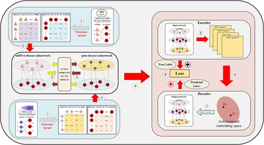
The overall framework of model MTLMDA.
In MTLMDA (see Figure 3 and Algorithm 1), Step I constructs miRNA–disease sub-network and gene–disease sub-network and to form a heterogeneous graph; Step II projects the corresponding disease and miRNA nodes, disease and gene nodes in each sub-network to the same vector space; Step III extracts the initial joint features of the two sub-networks as their auxiliary information; Step IV uses a graph convolutional network to get the embeddings of two sub-network nodes; Step V simultaneously feeds the node embeddings obtained in the two sub-networks into the linear decoder to reconstruct the links of two sub-networks; and Step (VI) trains the entire model by an end-to-end manner using the cross-entropy loss function of the integrated two sub-networks. In the following, we will elaborate the six steps in great details.
Step I: As introduced in Section of The Construction of Subnetworks, in miRNA–disease sub-network, there are |$495$| miRNA nodes and |$383$| disease nodes. From HMDD v.2.0, we can get |$5430$| experimentally verified miRNA–disease associations, which are treated as positive samples (with label value |$1$|). As previous studies [38, 46], we randomly select miRNA–disease pairs from all the unknown miRNA–disease associations (marked as |$0$| in |$MD$|) as negative samples (with label value |$0$|). In addition, we introduce Gaussian similarity as the node feature of miRNA–disease sub-network. Therefore, node feature of |$i$|-th miRNA, |$M(i)$| can be expressed as a 495-dimension vector:
where |$x^{1}_{i,j}$| represents the Gaussian similarity between miRNA |$m_{i}$| and miRNA |$m_{j}$| in the miRNA–disease sub-network. Similarly, the node feature of |$i$|-th disease, |$D_{1}(i)$|, can be expressed as a 383-dimension vector:
where |$z_{i,j}$| represents the Gaussian similarity between disease |$d_{i}$| and disease |$d_{j}$|.
In gene–disease sub-network, we mine the associated gene–disease pairs in terms of diseases in miRNA–disease sub-network from the DisGeNet database. There are |$9286$| associations (i.e. positive samples with label value |$1$|) between |$n_{d}$| diseases and |$n_{g}$| genes. We randomly select the gene–disease pairs from all the unknown disease-gene associations (marked as |$0$| in |$GD$|) to form negative samples (with label value |$0$|). We also deploy Gaussian similarity as initial features for gene and disease nodes, |$G(i)$| (feature vector of gene |$g_{i}$|) and |$D_{2}(\,j)$| (feature vector of disease |$d_{i}$|), can be expressed as follows respectively:
where |$x^{2}_{i,j}$| represents the Gaussian similarity between gene |$g_{i}$| and |$g_{j}$|, and |$z^{2}_{i,j}$| represents the Gaussian similarity between disease |$d_{i}$| and disease |$d_{j}$| in the gene–disease sub-network.
Step II: In the two sub-networks, nodes possess feature vectors of varying dimensions. To streamline the calculation process in subsequent steps, we have developed a projection module that unifies disparate node features into a common vector space. Specifically, in the miRNA–disease sub-network, the projection module maps disease and miRNA node features to a uniform 1024-dimensional space via a transition matrix. The process is as follows:
where |$H_{m}(i)\in \mathbb{R}^{1024}$| and |$H_{d1}(i)\in \mathbb{R}^{1024}$| are projection features of miRNA node |$m_{i}$| and disease node |$d_{i}$| in miRNA–disease network. Likewise, |$H_{g}(i)\in \mathbb{R}^{1024}$| and |$H_{d2}(i)\in \mathbb{R}^{1024}$| are projection features of gene |$g_{i}$| and disease |$d_{i}$| in the gene–disease network. The learnable weight matrices |$\mathbf{W}_{m}\in \mathbb{R}^{495\times 1024}$|, |$\mathbf{W}_{g}\in \mathbb{R}^{4395\times 1024}$| and |$\mathbf{W}_{d}\in \mathbb{R}^{383\times 1024}$| are automatically generated by calling the torch package, according to the size requirements of our designed space vector. In order to reduce redundant parameters and learning time in the experiment, here, the weight matrix |$\mathbf{W}_{d}\in \mathbb{R}^{383\times 1024}$| is used to share to complete the task of mapping the disease nodes to the latent space in the two networks.
Step III: In this step, we connect the two sub-networks through cross&compress units module and simultaneously extract the auxiliary information from both sub-networks by analyzing the MD and GD matrices. |$\mathbf{H}_{aux-m}\in \mathbb{R}^{495\times 1024}$| and |$\mathbf{H}_{aux-d1}\in \mathbb{R}^{383\times 1024}$| respectively represent the miRNA and disease nodes in the miRNA–disease network, which have obtained auxiliary information from their own network and the gene–disease network.
The weight matrices, |$\mathbf{W}_{aux-m}\in \mathbb{R}^{383\times 1024}$| and |$\mathbf{W}_{aux-d1}\in \mathbb{R}^{4395\times 1024}$|, are automatically generated using the Torch package to extract auxiliary information from corresponding networks. A similar process occurred in the gene–disease network is as follows:
Ultimately, we concatenate the initial features of the nodes with the auxiliary features to form the new features of the nodes, which can be summarized as follows:
where |$\mathbf{H}_{M}\in \mathbb{R}^{495\times 2048}$| and |$\mathbf{H}_{D1}\in \mathbb{R}^{383\times 2048}$| represent the integrated feature representations of nodes in the miRNA–disease network, while |$\mathbf{H}_{G}\in \mathbb{R}^{4935\times 2048}$| and |$\mathbf{H}_{D2}\in \mathbb{R}^{383\times 2048}$| represent integrated gene and disease nodes features in gene–disease sub-network respectively.
Step IV: Here, we further obtain the representations of two sub-network nodes using information about their direct neighbors in their respective networks based on graph convolutional network (GCN) encoder. Here, we adopt the Chebyshev filter-based approach (ChebConv) as MTLMDA’s encoder in view of its great expressive power [47]. At each layer of a graph convolutional network, MTLMDA update nodes’ embeddings according to the edges in the respective sub-networks (take the miRNA–disease sub-network as an example):
where |$\mathbf{h}_{i}^{(l)}\in \mathbb{R}^{u}$| represents the hidden state of node |$i$| at the |$l$|-th layer of the GCN (|$u$| is the dimension of hidden state representation), and |$\mathbf{W}$| is learnable weight. In the study, |$k$| is the Chebyshev filter size (being set to 2 here). |$\widetilde{\mathbf{A}}\in \mathbb{R}^{(n_{d}+n_{m})\times (n_{d}+n_{m})}=\mathbf{A}_{MD}+\mathbf{I}$|, where |$A_{MD}$| is the adjacency matrix of the miRNA–disease sub-network. |$\widetilde{\mathbf{D}}$| is the diagonal degree matrix of |$\widetilde{\mathbf{A}}$| with |$D_{ii}=\sum _{j}a_{i,j}$| (|$a_{i,j}$| denotes corresponding entry value of matrix |$\widetilde{\mathbf{A}}$|). |$\lambda _{max}$| is the largest eigenvalue of |$\mathbf{L}$|. With the above Cheb-GCN encoder, we get the embeddings of the nodes in the two sub-network the final, respectively.
Step V: After obtaining the node representations of the two sub-networks, we then employ a linear decoder to reconstruct the links of heterogeneous graphs in the two sub-networks. The detailed representation is as follows:
where |$\hat{y}_{md}$| represents the predicted association probability of miRNA node |$m(i)$| and disease node |$d(\,j)$| in the miRNA–disease sub-network, |$F_{m}$| and |$F_{d1}$| represent the final miRNA and disease node embedding representations obtained through the MTLMDA encoder respectively in the miRNA–disease sub-network, and |$Q_{1}$| denotes a trainable parameter matrix, which is 64*64 dimensions. Sigmoid function represents:
similarly, |$\hat{y}_{gd}$| represents the predicted association probability of gene nodes and the disease nodes in the gene–disease sub-network.
Step VI: The loss function of MTLMDA model is the sum of reconstructed errors from all training samples in the two sub-networks. Here, we choose the cross-entropy loss function to measure the error between the ture vaule |$y$| of each associations in the sub-network and predicted probability value |$\hat{y}$|. The form is as follows:
where |$LOSS_{m-d}$| represents the functional loss in the miRNA–disease sub-network, |$\hat{y}_{ij}$| represents the predicted link probability between disease and miRNA nodes, while |$y_{ij}$| represents the true label of the link, which will be 1 or 0. Correspondingly, |$LOSS_{g-d}$| represents the functional loss in the gene–disease sub-network. We take the sum of the two sub-network losses as the loss of MTLMDA whose form is as follows:
Then, we use the Loss function in Eq. (31) to train the whole model via back propagation algorithm with an end-toend manner.
RESULTS
In this section, we show the comparison results under different experimental conditions and different models on HMDD v2.0 dataset [41] to demonstrate the effectiveness of our proposed MTLMDA model.
Implementation settings
MTLMDA is implemented in the pytorch(v1.10.2) framework based on the DGL(v0.6.1) platform [48]. During model training, model parameters are randomly initialized and optimized with Adam. We adopted grid search to find the MTLMDA’s optimal hyper parameters, the learning rate is set to 0.0001 and the weight decay is set to 3*|$10^{-4}$|. In order to prevent the overfitting, we add a drop mechanism in the model [38]. We select different dropout rates from 0.1 to 0.9 during the training process and the model performs the best when dropout rate is 0.3. The entire model is trained 800 epochs and output the test set results every 10 epochs. Please see Table 2 for the detailed hyperparameter settings in our experiment. The 5-fold cross-validation is applied to the performance evaluation of MTLMDA. In 5-fold cross-validation, the sample dataset is randomly divided into five subsets. At each time, one subset of data is used as the test set and the remaining four sets of subsets are used as the training set. After repeating the similar process five times, we can obtain the objective and fair experimental evaluation results.
Setting of hyperparameters
| Model | Hyper-parameter | HMDD v2.0 | Searching space | Description |
|---|---|---|---|---|
| MTLMDA | Weight|$\_$|decay | |$3*10^{-4}$| | |$[10^{-3},10^{-4},3*10^{-4},10^{-5}]$| | |$L_{2}$| regularization coefficient. |
| Layers | 3 | |$[1,2,3,4,5]$| | Number of layers of chebGCN. | |
| Dropout | 0.3 | |$[0.1-0.9]$| | Dropout rate. | |
| |$lr$| | |$10^{-4}$| | |$[10^{-2},10^{-3},5*10^{-4},10^{-4},10^{-5}]$| | Learning rate. | |
| Projection dimension | 1024 | |$[64,128,256,512,1024,2048]$| | Node feature mapping dimension. | |
| Embedding dimension | 64 | |$[16,32,64,128,256,512]$| | Node feature embedding dimension. |
Evaluation metrics
To comprehensively evaluate the performance of our proposed MTLMDA, we choose Precision (Prec.), Accuracy (Acc.), Recall, F1 score, AUC and precision–recall (P–R) curve as the evaluation criteria. The corresponding mathematical calculation is represented as follows:
where |$TP$|, |$FP$|, |$TN$| and |$FN$| denote true positive, false positive, true negative and false negative, respectively. AUC refers to the area under the receiver operating characteristic (ROC) curve, which can quantitatively reflect the model performance measured based on the ROC curve. The abscissa of |$ROC$| curve represents |$FPR$| and the ordinate is |$TPR$| where |$TPR$| and |$TPR$| are calculated as follows:
The abscissa of the P–R curve represents the recall of the model and the ordinate represents the precision. The larger area in the P–R curve represents better model performance. Table 3 describes the values of various evaluation indicators of our model using 5-fold cross-validation in detail.
5-fold cross-validation results performed
| Test set | Precision | Accuracy | Recall | F1-score |
|---|---|---|---|---|
| 1 | 0.8730 | 0.8656 | 0.8831 | 0.8670 |
| 2 | 0.8762 | 0.8743 | 0.8745 | 0.8733 |
| 3 | 0.8520 | 0.8780 | 0.8537 | 0.8751 |
| 4 | 0.8903 | 0.8660 | 0.8756 | 0.8697 |
| 5 | 0.8899 | 0.8600 | 0.8630 | 0.8598 |
| Mean | 87.63% |$\,\pm\, $|0.0046 | 86.88% |$\,\pm\, $|0.0065 | 87.74% |$\,\pm\, $|0.0104 | 86.93% |$\,\pm\, $|0.0054 |
We observe that MTLMDA has achieved an average Accuracy of 86.88%, Precision of 87.63%, Recall of 87.74% and F1 score of 86.93%. Moreover, Figure 4 shows that the AUC values of MTLMDA’s ROC curves under five-fold cross-validation are: 94.03%, 94.67%, 93.75%, 94.62%, 93.79%, with an average of 94.17% |$\,\pm\, $|0.0040. At the same time, Figure 5 shows that the values AUC of MTLMDA’s P–R curve under 5-fold cross-validation are: 93.27%, 93.53%, 94.55%, 94.10% and 93.31% with an average of 93.75% |$\,\pm\, $| 0.0050. To further demonstrate the value of incorporating gene–disease information in MTLMDA, we conducted an experiment whereby the miRNA–disease network remained unchanged while the gene–disease network was randomly shuffled, disrupting the original associations between genes and diseases. The validation results are shown in Table 4. Interestingly, despite the randomization of the gene–disease network, it is still possible for the two networks to exhibit similar structures within the vector space of disease nodes during the initial non-specific task of multi-task learning [22]. As a result, the perturbed gene–disease network can still offer significant auxiliary information to the miRNA–disease network.
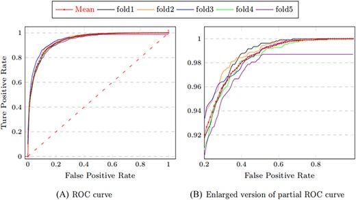
ROC curves of MTLMDA in 5-fold cross validation.
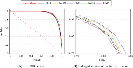
P–R curves of MTLMDA in 5-fold cross validation.
5-fold cross-validation (random shuffle gene–disease associations) performed
| Test set | 1 | 2 | 3 | 4 | 5 | Mean |
|---|---|---|---|---|---|---|
| Precision | 0.8561 | 0.8552 | 0.8496 | 0.8369 | 0.8427 | 84.81%|$\,\pm\, $|0.0074 |
| Accuracy | 0.8487 | 0.8565 | 0.8620 | 0.8638 | 0.8500 | 85.62%|$\,\pm\, $|0.0061 |
| Recall | 0.8249 | 0.8377 | 0.8528 | 0.8765 | 0.8379 | 84.60%|$\,\pm\, $|0.0176 |
| F1-score | 0.8350 | 0.8464 | 0.8512 | 0.8562 | 0.8403 | 84.58%|$\,\pm\, $|0.0076 |
| AUC | 0.9275 | 0.9362 | 0.9265 | 0.9340 | 0.9284 | 93.05%|$\,\pm\, $|0.0039 |
Comparison with other latest methods
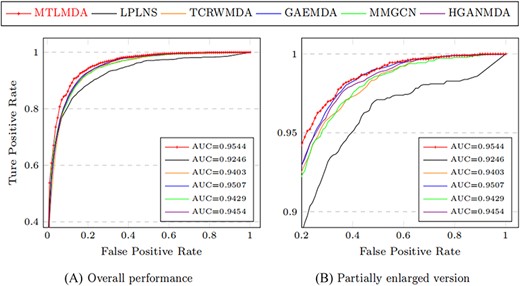
The constructed training samples are data sets with balanced positive and negative samples. Therefore, the ROC curve can more intuitively show the performance of the model. Here, we use the AUC values based on the ROC curve to compare the performance of MTLMDA with the other state-of-the-art models in a 5-fold cross-validation manner. We have selected the latest and most representative models in this field, which are ”Predicting microRNA–disease associations using label propagation based on linear neighborhood similarity” (LPLNS) [27], ”Tree-layer heterogeneous network combined with unbalanced random walk for miRNA–disease association prediction” (TCRWMDA)[31], ”A graph auto-encoder model for miRNA–disease associations prediction” (GAEMDA) [38], ”Multi-view multichannel attention graph convolutional network for miRN–disease association prediction” (MMGCN) [49] and ”Hierarchical graph attention network for miRNA–disease association prediction” (HGANMDA) [46]. For fair experiments, the five comparison algorithms are all performed 5-fold cross-validation experiments on HMDD v2.0 dataset. Figure 6 shows the ROC curve comparison of MTLMDA with the other five contrasting algorithms. In addition, Figure 7 compares our method with other approaches using an alternative version of the 5-fold cross-validation. Unlike the standard 5-fold cross-validation where the dataset is randomly partitioned, we used the average Gaussian similarity of each miRNA node with respect to the disease to divide the dataset into five parts. Table 5 shows the AUC values for each model in different versions of 5-fold cross-validation based on the HMDD V2.0. As shown in Figure 8, to obtain a more comprehensive evaluation, we further use the data of HMDD V2.0 as training, and use the data set of HMDD V3.2 [50] for test comparison. From the results, we observe that our MTLMDA perform better than the baseline methods. Comparing to other models, MTLMDA fully takes into account the relatively sparse relationships between miRNAs and diseases on the database and utilizes multi-task learning to effectively explore the sparse relationships. Moreover, MTLMDA uses the information of gene–disease network to assist the prediction of miRNA–disease improving the overall performance of the model. Therefore, MTLMDA achieves excellent results.
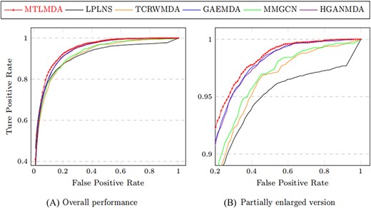
Comparison of ROC curves in 5-fold cross validation based on HMDD v2.0.
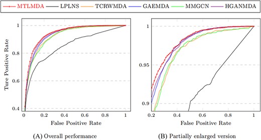
Comparison of ROC curves based on the alternative version of the 5-fold cross-validation.
Comparison of ROC curves based on the HMDD v3.2.
5-fold cross-validation results comparison
| Models | AUC | AUC (alternative version) |
|---|---|---|
| LPLNS | 0.9107|$\,\pm\, $|0.0041 | 0.8524|$\,\pm\, $|0.0018 |
| TCRWMDA | 0.9209|$\,\pm\, $|0.0036 | 0.9157|$\,\pm\, $|0.0033 |
| GAEMDA | 0.9356|$\,\pm\, $|0.0044 | 0.9319|$\,\pm\, $|0.0049 |
| MMGCN | 0.9266|$\,\pm\, $|0.0022 | 0.9191|$\,\pm\, $|0.0015 |
| HGANMDA | 0.9374|$\,\pm\, $|0.0041 | 0.9336|$\,\pm\, $|0.0038 |
| MTLMDA | 0.9417|$\,\pm\, $|0.0040 | 0.9404|$\,\pm\, $|0.0039 |
Performance analysis of the model under different feature information
To further demonstrate the effectiveness of our proposed model, we conduct ablation experiments. Our model is experimented with Gaussian features and auxiliary features(AUX+GUS), only Gaussian features(GUS), only auxiliary features(AUX) and only original edge features(Edge). Table 6 shows the model performance under different node features and visualized in Figure 9.
Performance comparison of models under different node information
| Node feature | AUC (%) | Precision (%) | Accuracy (%) | Recall (%) | F1-score (%) |
|---|---|---|---|---|---|
| Edge | 91.22 | 83.37 | 83.58 | 83.90 | 83.63 |
| AUX | 90.73 | 85.37 | 84.38 | 81.43 | 83.91 |
| GUS | 92.15 | 84.20 | 85.32 | 80.74 | 83.62 |
| AUX+GUS | 94.17 | 86.13 | 86.88 | 87.74 | 86.93 |
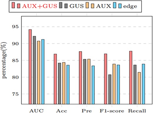
Comparing the results under different node features (AUX+GUS, GUS,AUX, edge represents the performance of the model under Gaussian similarity and auxiliary information, only Gaussian similarity, only auxiliary information, and only edge information, respectively).
Performance analysis of the model under different GCN layers
In the encoder of MTLMDA, we aggregate the information of the network through the GCN, and then generate the representation of the network nodes. The different number of GCN layers in the encoder will lead to different aggregation effects on the node information in the network, which will affect the final prediction performance of the model. Figure 10A shows the performance of our model for different numbers of GCN layers in the encoder. We see that the performance of MTLMDA reaches the best performance when the number of GCN layers is 3 in the encoder, while the number of layers is ¿3, the performance will drop rapidly. We know that the |$0th$| layer embedding of a node in encoder is its input feature, |$layer-k$| embedding obtains information from nodes that are |$k$| hops away on the formed heterogeneous graph. If the encoder of the model contains an excessive number of GCN layers, every node in graph will obtain highly overlapped node information. As a result, the model suffers from the over-smoothing problem. As shown in Figure 10A, when the number of GCN layers is greater than 3, the model performance begins to degrade.
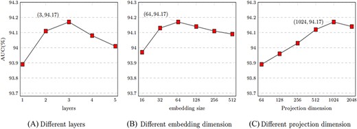
The value of MTLMDA under different experimental parameters.
Performance analysis of the model under different embedding dimension
The size of the embedding representation of the nodes obtained after encoding by the MTLMDA encoder is an important factor affecting the performance of the model. The size of different node embeddings contains different node information for the same node. In the experiment, we choose the size of node embedding dimension as 16, 32, 64, 128, 256 and 512 respectively. In Figure 10B, the overall performance of the model is constantly improved within a certain range over the node embedding dimension. When the embedding dimension reaches 64, the performance of the model is the best. Thus, we choose 64 dimensions as the default embedding dimension of MTLMDA encoder.
Performance analysis of the model under different projection dimension
The projection dimension of the network nodes in the model is the most important factor in determining the initial characteristics of the nodes in the model encoder. For the experiments, we explore the performance of the model under different projection dimensions based on a 3-layer GCN encoder. As demonstrated in Figure 10C, we set the projection dimensions to 64, 128, 256, 512, 1024, and 2048, respectively. The experimental results show that the overall performance of the model is the optimal when the projection dimension is 1024. Therefore, in subsequent experiments, we choose 1024 as the default value of the projection dimension.
Comprehensive comparison of different models
To further demonstrate the comprehensive performance of MTLMDA, we regard the model as a recommender system, where miRNAs represent users and diseases represent items. Our task is to determine whether there is an interaction between the user and different items. Therefore, we conduct the experiment by using all known associateds in HDMM v2.0 as the training samples to identify various top rankings miRNAs for each diseases. Here, we mainly focus on the number of predicted positive samples in the different top-ranked. Figure 11 shows the numbers of correctly retrieved miRNA–disease associations. We observe that MTLMDA outperforms the other models among top 5 to top 50.
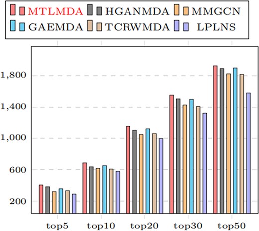
Number of correctly retrieved known miRNA–disease associations of top-k.
Real case studies for the proposed MTLMDA
To further test the predictive ability of MTLMDA for potentially disease-miRNA associations in practice, we leverage the model to conduct case studies on six common malignant human diseases. We learn that approximately 200 miRNAs have been found to be significantly dysregulated in various cancer malignancies. These miRNAs can produce effect on cancer generation by targeting proto-oncogenes or tumor suppressor genes [51]. Therefore, accurate prediction of potential miRNA–disease associations is a major advance in the field of human medicine and health. During the prediction process of the model, the training set of miRNA–disease sub-network includes positive samples of 5430 experimentally confirmed miRNA–disease combinations and the same number of negative samples randomly selected from the miRNA–disease combinations. And then, we establish the corresponding gene–disease sub-network training set according to the diseases in the miRNA–disease sub-network. The test set of MTLMDA is assembled through the disease of case studied with the remaining miRNAs in the miRNA–disease sub-network. By training the MTLMDA, we can get embedded representations for diseases and miRNAs. By decoding the test set, we can get the association probability between the disease and remaining miRNAs. For each disease, we select the top 30 miRNAs with the highest predicted association probability scores. For the prediction results, we use the three databases (i.e. dbDEMC [52], miR2Disease [53] and miRCancer [54]) to verify them in turn. If the results are confirmed in dbDEMC, we will no longer query the miR2Disease and miRCancer databases. Otherwise, we query them sequentially.
Lung cancer is the most common cause of death among all cancer pathologies. Most patients are not noticed until advanced-stage, and the prognosis is generally poor [55]. We know that loss or amplification of some miRNAs has been found the association with lung cancer. Therefore, it is very necessary to design the case study to explore potential associated miRNA in lung cancer. From Table 7, we observe that 29 of the top 30 candidate miRNAs can be confirmed with the three databases. Specifically, there is no evidence that hsa-mir-378a is associated with lung cancer, perhaps the connection has not been discovered yet rather than confirming no link.
Top 30 lung cancer-related miRNAs predicted
| Rank | miRNA | Evidence | Rank | miRNA | Evidence |
|---|---|---|---|---|---|
| 1 | hsa-mir-16 | dbDEMC | 16 | hsa-mir-378a | NO |
| 2 | hsa-mir-122 | dbDEMC | 17 | hsa-mir-99a | dbDEMC |
| 3 | hsa-mir-15a | dbDEMC | 18 | hsa-mir-302a | dbDEMC |
| 4 | hsa-mir-106b | dbDEMC | 19 | hsa-mir-328 | dbDEMC |
| 5 | hsa-mir-15b | dbDEMC | 20 | hsa-mir-196b | dbDEMC |
| 6 | hsa-mir-195 | dbDEMC | 21 | hsa-mir-372 | dbDEMC |
| 7 | hsa-mir-141 | dbDEMC | 22 | hsa-mir-483 | dbDEMC |
| 8 | hsa-mir-451a | dbDEMC | 23 | hsa-mir-10a | dbDEMC |
| 9 | hsa-mir-23b | dbDEMC | 24 | hsa-mir-208a | dbDEMC |
| 10 | hsa-mir-342 | dbDEMC | 25 | hsa-mir-424 | mirCancer |
| 11 | hsa-mir-429 | dbDEMC | 26 | hsa-mir-302b | dbDEMC |
| 12 | hsa-mir-373 | dbDEMC | 27 | hsa-mir-204 | dbDEMC |
| 13 | hsa-mir-20b | dbDEMC | 28 | hsa-mir-144 | dbDEMC |
| 14 | hsa-mir-130a | dbDEMC | 29 | hsa-mir-28 | dbDEMC |
| 15 | hsa-mir-193b | dbDEMC | 30 | hsa-mir-149 | dbDEMC |
Colon cancer is a type of cancer that begins in the large intestine (Colon). The colon is the final part of the digestive tract. Colon cancer can occur at any age but it is more likely to affect older adults. It usually starts as small noncancerous (benign) clumps of cells called polyps that form inside the colon. Some of these polyps can turn into colon cancer over time. An estimated 106 180 colon cancer cases will be diagnosed in the USA by 2022 [56]. From Table 8, the top 30 colon cancer-related miRNAs predicted by our model are confirmed on the three databases.
Top 30 colon cancer-related miRNAs predicted
| Rank | miRNA | Evidence | Rank | miRNA | Evidence |
|---|---|---|---|---|---|
| 1 | hsa-mir-21 | dbDEMC | 16 | hsa-mir-29c | dbDEMC |
| 2 | hsa-mir-155 | dbDEMC | 17 | hsa-mir-15b | miR2Disease |
| 3 | hsa-mir-34a | dbDEMC | 18 | hsa-mir-223 | dbDEMC |
| 4 | hsa-mir-146a | dbDEMC | 19 | hsa-mir-199a | mirCancer |
| 5 | hsa-mir-125b | dbDEMC | 20 | hsa-mir-19b | dbDEMC |
| 6 | hsa-mir-122 | dbDEMC | 21 | hsa-let-7a | dbDEMC |
| 7 | hsa-mir-16 | dbDEMC | 22 | hsa-mir-143 | dbDEMC |
| 8 | hsa-mir-221 | dbDEMC | 23 | hsa-mir-92a | dbDEMC |
| 9 | hsa-mir-29a | dbDEMC | 24 | hsa-mir-31 | dbDEMC |
| 10 | hsa-mir-222 | dbDEMC | 25 | hsa-mir-210 | dbDEMC |
| 11 | hsa-mir-133a | dbDEMC | 26 | hsa-mir-200b | dbDEMC |
| 12 | hsa-mir-29b | dbDEMC | 27 | hsa-mir-206 | dbDEMC |
| 13 | hsa-mir-1 | dbDEMC | 28 | hsa-mir-19a | dbDEMC |
| 14 | hsa-mir-20a | dbDEMC | 29 | hsa-mir-18a | dbDEMC |
| 15 | hsa-mir-15a | dbDEMC | 30 | hsa-let-7c | dbDEMC |
Lymphomas start in immune system cells and can occur almost anywhere in the body. In 2022, there will be an estimated 89 010 new cases of lymphoma in the USA and 21 170 people will die from the disease [56]. Our prediction results for lymphoma-associated miRNAs are shown in Table 9. Among the top 30 candidate miRNAs, only hsa-mir-142 and hsa-mir-34c have no evidence to prove their association with Lymphoma on the three databases.
Top 30 lymphoma-related miRNAs predicted
| Rank | miRNA | Evidence | Rank | miRNA | Evidence |
|---|---|---|---|---|---|
| 1 | hsa-mir-125b | dbDEMC | 16 | hsa-mir-196a | dbDEMC |
| 2 | hsa-mir-29a | dbDEMC | 17 | hsa-mir-214 | dbDEMC |
| 3 | hsa-mir-34a | dbDEMC | 18 | hsa-mir-195 | dbDEMC |
| 4 | hsa-mir-221 | dbDEMC | 19 | hsa-mir-30a | dbDEMC |
| 5 | hsa-mir-222 | dbDEMC | 20 | hsa-mir-9 | dbDEMC |
| 6 | hsa-mir-29b | dbDEMC | 21 | hsa-mir-143 | dbDEMC |
| 7 | hsa-mir-133a | dbDEMC | 22 | hsa-mir-181b | dbDEMC |
| 8 | hsa-mir-199a | dbDEMC | 23 | hsa-let-7c | dbDEMC |
| 9 | hsa-mir-1 | dbDEMC | 24 | hsa-let-7a | dbDEMC |
| 10 | hsa-mir-223 | dbDEMC | 25 | hsa-mir-15b | dbDEMC |
| 11 | hsa-mir-145 | dbDEMC | 26 | hsa-mir-23a | dbDEMC |
| 12 | hsa-mir-106b | dbDEMC | 27 | hsa-mir-146b | dbDEMC |
| 13 | hsa-mir-142 | NO | 28 | hsa-let-7b | dbDEMC |
| 14 | hsa-mir-206 | dbDEMC | 29 | hsa-mir-34c | NO |
| 15 | hsa-mir-31 | dbDEMC | 30 | hsa-mir-106a | dbDEMC |
Breast cancer is the most common cancer worldwide and the leading cause of cancer-related deaths in women, accounting for 25% of all cancer cases and 15% of cancer-related deaths [57]. Table 10 is the prediction results of our model for the top 30 breast cancer-related miRNAs. From the results, we see that only 25 candidate miRNAs have been confirmed to be related to breast cancer, and the remaining five miRNAs of hsa-mir-509, hsa-mir-362,hsa-mir-485, hsa-mir-491 and hsa-mir-378a do not find evidence relevance on the three databases.
Top 30 breast cancer-related miRNAs predicted
| Rank | miRNA | Evidence | Rank | miRNA | Evidence |
|---|---|---|---|---|---|
| 1 | hsa-mir-150 | dbDEMC | 16 | hsa-mir-192 | dbDEMC |
| 2 | hsa-mir-15b | dbDEMC | 17 | hsa-mir-491 | NO |
| 3 | hsa-mir-212 | dbDEMC | 18 | hsa-mir-95 | dbDEMC |
| 4 | hsa-mir-509 | NO | 19 | hsa-mir-154 | dbDEMC |
| 5 | hsa-mir-503 | dbDEMC | 20 | hsa-mir-483 | dbDEMC |
| 6 | hsa-mir-142 | miR2Disease | 21 | hsa-mir-184 | dbDEMC |
| 7 | hsa-mir-106b | dbDEMC | 22 | hsa-mir-720 | dbDEMC |
| 8 | hsa-mir-372 | dbDEMC | 23 | hsa-mir-431 | dbDEMC |
| 9 | hsa-mir-362 | NO | 24 | hsa-mir-363 | dbDEMC |
| 10 | hsa-mir-32 | dbDEMC | 25 | hsa-mir-28 | mirCancer |
| 11 | hsa-mir-208a | dbDEMC | 26 | hsa-mir-193a | dbDEMC |
| 12 | hsa-mir-485 | NO | 27 | hsa-mir-378a | NO |
| 13 | hsa-mir-30e | dbDEMC | 28 | hsa-mir-198 | dbDEMC |
| 14 | hsa-mir-190a | dbDEMC | 29 | hsa-mir-424 | dbDEMC |
| 15 | hsa-mir-98 | dbDEMC | 30 | hsa-mir-186 | dbDEMC |
Kidney Cancer is one of the 10 most common cancers in the Western community. Globally, approximately 270 000 kidney cancer cases are diagnosed each year, and 116 000 of them die from the disease[58]. It can be seen from the results in Table 11 that the top 30 candidate miRNAs predicted by MTLMDA have all been confirmed the connection.
Top 30 kidney cancer-related miRNAs predicted
| Rank | miRNA | Evidence | Rank | miRNA | Evidence |
|---|---|---|---|---|---|
| 1 | hsa-mir-155 | dbDEMC | 16 | hsa-mir-223 | dbDEMC |
| 2 | hsa-mir-146a | dbDEMC | 17 | hsa-mir-126 | dbDEMC |
| 3 | hsa-mir-29a | dbDEMC | 18 | hsa-mir-199a | dbDEMC |
| 4 | hsa-mir-34a | dbDEMC | 19 | hsa-mir-18a | dbDEMC |
| 5 | hsa-mir-125b | dbDEMC | 20 | hsa-mir-143 | dbDEMC |
| 6 | hsa-mir-122 | dbDEMC | 21 | hsa-mir-19b | dbDEMC |
| 7 | hsa-mir-221 | dbDEMC | 22 | hsa-mir-150 | dbDEMC |
| 8 | hsa-mir-16 | dbDEMC | 23 | hsa-mir-19a | dbDEMC |
| 9 | hsa-mir-133b | dbDEMC | 24 | hsa-mir-92a | dbDEMC |
| 10 | hsa-mir-20a | dbDEMC | 25 | hsa-mir-15b | dbDEMC |
| 11 | hsa-mir-17 | dbDEMC | 26 | hsa-mir-31 | dbDEMC |
| 12 | hsa-mir-29b | dbDEMC | 27 | hsa-mir-7a | dbDEMC |
| 13 | hsa-mir-222 | mirCancer | 28 | hsa-mir-195 | dbDEMC |
| 14 | hsa-mir-1 | dbDEMC | 29 | hsa-mir-181a | dbDEMC |
| 15 | hsa-mir-145 | dbDEMC | 30 | hsa-mir-200b | dbDEMC |
Leukemia is a cancer of the bone marrow and blood. From 2009 to 2018, the incidence of leukemia in children and adolescents increased by about 1% per year [56]. We choose Leukemia as our final set of case studies. Table 12 shows the top 30 miRNAs predicted by our model that may be associated with Leukemia, and then the prediction results are confirmed through the three datasets.
Top 30 leukemia-related miRNAs predicted
| Rank | miRNA | Evidence | Rank | miRNA | Evidence |
|---|---|---|---|---|---|
| 1 | hsa-mir-155 | dbDEMC | 16 | hsa-mir-34c | dbDEMC |
| 2 | hsa-mir-146a | dbDEMC | 17 | hsa-mir-200b | dbDEMC |
| 3 | hsa-mir-29a | dbDEMC | 18 | hsa-mir-200a | dbDEMC |
| 4 | hsa-mir-221 | dbDEMC | 19 | hsa-mir-206 | dbDEMC |
| 5 | hsa-mir-133a | dbDEMC | 20 | hsa-let-7a | dbDEMC |
| 6 | hsa-mir-122 | miRCancer | 21 | hsa-let-7d | dbDEMC |
| 7 | hsa-mir-222 | dbDEMC | 22 | hsa-mir-182 | dbDEMC |
| 8 | hsa-mir-29b | dbDEMC | 23 | hsa-mir-146b | dbDEMC |
| 9 | hsa-mir-145 | dbDEMC | 24 | hsa-let-7e | dbDEMC |
| 10 | hsa-mir-1 | dbDEMC | 25 | hsa-mir-195 | dbDEMC |
| 11 | hsa-mir-106b | dbDEMC | 26 | hsa-mir-142 | dbDEMC |
| 12 | hsa-mir-223 | dbDEMC | 27 | hsa-mir-210 | dbDEMC |
| 13 | hsa-mir-126 | dbDEMC | 28 | hsa-mir-148a | dbDEMC |
| 14 | hsa-mir-15b | dbDEMC | 29 | hsa-mir-26a | dbDEMC |
| 15 | hsa-mir-29c | dbDEMC | 30 | hsa-mir-106a | dbDEMC |
From the above six groups of case studies, we can further confirm the reliability of our model. In summary, we provide a reliable reference and guidance for miRNA-disease association research through our proposed model.
CONCLUSION
Various malignant diseases in humans are formed in the process of miRNAs controlling gene expression and abnormal expression of miRNAs is a key element of human diseases. Therefore, accurate relationship prediction between diseases and miRNAs can promote the progress of human health. In this paper, we propose multi-task learning model (i.e. MTLMDA) to predict potential miRNA–disease associations. According to the diseases in the miRNA–disease network, we construct the corresponding gene–disease sub-network to assist the prediction task of miRNA–disease associations. Compared with five latest classic benchmark models, our proposed MTLMDA model obtains superior AUC. Moreover, the accuracy and reliability of MTLMDA model in the prediction process are confirmed through six case studies (lung cancer, colon cancer, lymphoma, breast cancer, kidney cancer and leukemia).
This is the first work (called MTLMDA) in the field to introduce the idea of multi-task learning through the use of miRNA–disease–gene relationships.
We select the same disease and related genes from the DisGeNet as the corresponding miRNA–disease sub-network to built the genes–disease sub-network, which was used to assist the miRNA–disease relationship prediction.
MTLMDA is an end-to-end trainable graph neural network model using GCN-based autoencoder and decoder.
we compare our model with competitive baselines on a real-world dataset and conduct six case studies for both miRNAs and diseases, which confirmed the effectiveness of our model.
FUNDING
National Natural Science Foundation of China (Grant No. 62202089, U22A2004, 72192832); Shanghai Rising-Star Program (Grant No. 23QA1403100); Natural Science Foundation of Shanghai (Grant No. 21ZR1421900); General project of Liaoning Provincial Department of Education (Grant No. LJKZ0005); Doctor Startup Foundation of Liaoning Province (Grant No. 2021-BS-055), Fundamental Research Funds for the Central Universities (Grant No. N2119004).
DATA AVAILABILITY
The data and source code are available from https://github.com/qwslle/MTLMDA.
Author Biographies
Qiang He received the Ph.D. degree in computer application technology from the Northeastern University, Shenyang, China in 2020. He is currently Associate Professor at College of Medicine and Biological Information Engineering, Northeastern University, Shenyang, China.
Wei Qiao is currently pursuing a master’s degree in electronic information from the Northeastern University, Shenyang, China. His main research interests are data mining, medical informatics.
Hui Fang is an Associate Professor at Shanghai University of Finance and Economics, China. She received her PhD from Nanyang Technological University, Singapore. Her main research topic is personalized machine learning, including trust/link prediction in online communities, and recommender systems. She has published papers in leading conferences (e.g., IJCAI, AAAI and SIGIR), and journals (e.g., AIJ, TKDE, TOIS and TPAMI). She is the SE of the ECRA journal, and serves as a PC Board of IJCAI, and (Senior) PC Member for WWW, UMAP, IJCAI, AAAI and AAMAS, etc.
Yang Bao received Ph.D. degree in Information Systems from the School of Computing at the National University of Singapore, and bachelor & master degree from Nanjing University. He is currently an Associate Professor at the Antai College of Economics and Management (ACEM), Shanghai Jiao Tong University (SJTU), Shanghai, China.
REFERENCES
