


Abstract
Spatially resolved transcriptomics (SRT) enable the comprehensive characterization of transcriptomic profiles in the context of tissue microenvironments. Unveiling spatial transcriptional heterogeneity needs to effectively incorporate spatial information accounting for the substantial spatial correlation of expression measurements. Here, we develop a computational method, SpaSRL (spatially aware self-representation learning), which flexibly enhances and decodes spatial transcriptional signals to simultaneously achieve spatial domain detection and spatial functional genes identification. This novel tunable spatially aware strategy of SpaSRL not only balances spatial and transcriptional coherence for the two tasks, but also can transfer spatial correlation constraint between them based on a unified model. In addition, this joint analysis by SpaSRL deciphers accurate and fine-grained tissue structures and ensures the effective extraction of biologically informative genes underlying spatial architecture. We verified the superiority of SpaSRL on spatial domain detection, spatial functional genes identification and data denoising using multiple SRT datasets obtained by different platforms and tissue sections. Our results illustrate SpaSRL’s utility in flexible integration of spatial information and novel discovery of biological insights from spatial transcriptomic datasets.
INTRODUCTION
Recent advances in spatially resolved transcriptomics (SRTs) have enabled high-throughput sequencing of mRNA coupled with spatial information in multicellular organisms, which can resolve cellular localizations to unveil the organizational landscape of complex tissues [1]. The SRT sequencing-based techniques, such as spatial transcriptomics (STs) [2], 10× Visium, Slide-seqV2 [3], can measure the expression level of tens of thousands of genes in thousands of tissue locations (or spots), which enables the comprehensive study of spatial transcriptional landscape from tissue architecture heterogeneity and the corresponding functional genes. However, SRT measurements are often sparse and noisy due to various technical limitations e.g. transcript capture rate or spatial resolution, which pose great challenges to decipher the spatially functional regions and genes [4]. Apart from dimension reduction, an effective usage of the locational information contained in SRT data can also mitigate data noise or bias, improving the pattern recognition in SRT studies, as neighbouring locations on tissue often share cell microenvironments and display similar gene expression levels in STs [5].
To resolve tissue structure, spatial domain detection is an important research topic, which aims to cluster spots with similar gene expression and spatial continuity within each cluster (or spatial domain). For this purpose, several currently presented spatial clustering approaches e.g. BayesSpace [6], Hidden Markov Random Field [7], SEDR [8], STAGATE [9] and SpaGCN [10], additionally constrain the models with spatial information to facilitate the identification of spatial domains with spatial smoothness. Their outcomes display more spatially continuity than those from clustering methods previously developed for single-cell RNA-sequencing studies that only utilize expression measurements e.g. Seurat [11], SCANPY [12]. However, these methods often take spatial neighbour prior as a hard constraint to ensure spatial continuity in spatial domains, but seldom provide a flexible solution to balance spatial coherence and expression variability within neighbourhoods.
In addition, most existing methods substantially perform dimension reduction before clustering spots and the common approach is principal component analysis (PCA) that is adopted to preprocess SRT data by e.g. Seurat, SCANPY, BayesSpace, SEDR and SpaGCN. PCA or other linear dimension reduction techniques can not only mitigate data noise but also extract the potential functional genes from a co-expression or functional association perspective [13]. However, such use of dimension reduction for SRT studies does not ensure that the inferred components (or meta-genes) are relevant to the spatial map on the tissue. This may limit their effectiveness or biological interpretations. Whereas, some recent works have made efforts to deal with this issue. For example, SpatialPCA [5] incorporates spatial information to improve locational neighbourhood similarity in the constructed PC space. DR-SC [14] performs simultaneous clustering and dimension reduction for better biological associations between the detected clusters and (meta) genes. However, it is still challenging to unify the characterization of locational and gene patterns accounting for spatial coherence and biological interpretations in SRT studies.
To this end, we present spatially aware self-representation learning (SpaSRL), a novel method that achieves spatial domain detection and dimension reduction in a unified framework while flexibly incorporating spatial information. Specifically, SpaSRL enhances and decodes the shared expression between spots for simultaneously optimizing the low-dimensional spatial components (i.e. spatial meta genes) and spot–spot relations through a joint learning model that can transfer spatial information constraint from each other. SpaSRL can improve the performance of each task and fill the gap between the identification of spatial domains and functional (meta) genes accounting for biological and spatial coherence on tissue. Thus, SpaSRL not only deciphers fine-grained spatial domains and extracts spatial interpretable functional genes underlying spatial domains, but also corrects the low-quality gene expression from borrowing information within spatial clusters, which flexibly balances spatial coherence and expression variability.
We demonstrate the superiority of SpaSRL to identify accurate spatial domains and functional (meta) genes on datasets sequenced by different technologies. We illustrate that SpaSRL can flexibly exert spatial information on the identification of spatial domains and functional genes as complementary to the current usage of spatial information. Applied to breast cancer slices, SpaSRL deciphers intratumour heterogeneity and finds more novel cancer-associated genes, which are validated by the survival analysis of independent clinical data. Applied to brain slices, SpaSRL reveals the tissue structures and the corresponding functional genes for interpreting tissue functions.
METHODS
Overview of SpaSRL
SpaSRL first enhances the shared expression among spots by incorporating spatial information into gene expression (Figure 1A). SpaSRL borrows the shared information from spatially neighbouring spots to adjust gene expression in each spot (i.e. |$\textrm{original}\ \textrm{expression}\ \textrm{matrix}\ {X}^0\in{R}^{M\times N}\to \textrm{enhanced}\ \textrm{expression}\ \textrm{data}\ X\in{R}^{M\times N},M$| and |$N$|, respectively, denote the number of genes and spots), which can correct the low-quality expression measurements and enrich local signals. The parameter |$\alpha$| is set to flexibly control the spatial information constraint on gene expression measurements.
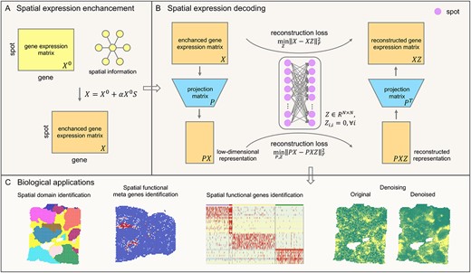
Schematic overview of SpaSRL enhancing-decoding (A&B) processes and potential applications of SpaSRL in downstream SRT analysis (C). (A) Spatial expression enhancement from aggregating expression information from neighbourhood spots. SpaSRL incorporates spatial information into gene expression to enhance the shared expression between spots by flexibly aggregating the weighed gene expression from their |$k$| spatial neighbors (e.g. |${X}^0\to X$|). |$S$| denotes the weight of expression similarity between each spot and its |$k$| neighbors. |$\alpha$| controls the contribution of spatial similarity to the enhanced expression measurements. (B) Spatial expression decoding via the feature extraction embedded self-representation learning model. The input data (i.e. |$X$|) is the enhanced gene expression matrix from (A). SpaSRL uses a robust projection matrix (i.e. |$P$|) to generate the low-dimensional representation (i.e. |$X\to PX,{P}^T PX=X$|). Based on the original and low-dimensional data, SpaSRL performs data reconstructions via an aggregated weight matrix |$Z$| based on self-representation learning algorithm (i.e. |$X= XZ$| and |$PX= PXZ$|). SpaSRL iteratively learns the projection matrix (i.e. |$P$|) and spot–spot similarity matrix (i.e. |$Z$|) by minimizing the sum of reconstruction losses (see Methods). When SpaSRL reaches convergence, the two optimal matrices are achieved for further downstream analyses. (C) Biological applications for SpaSRL including spatial domain identification, functional genes/meta genes identification and data denoising. The spot–spot similarity matrix can be applied to detect spatial domains and data denoising. The projection matrix can be employed to identify functional genes/meta genes to improve biological insights into tissue heterogeneity.
SpaSRL then decodes the spatially enhanced biological signals based on a novel self-representation learning model (Figure 1B). In the model, SpaSRL introduces an aggregated weight matrix |$Z\in{R}^{N\times N}$| and a projection matrix |$P$| (i.e. |$P\in{R}^{\textrm{d}\times M}$|, |$d\ll M$|, |$d$| is the number of meta genes) to reconstruct expression data as the linear combinations of expression measurements of similar locations in the original and low-dimensional feature spaces (i.e. |$X\to PX,$| |$X= XZ$| and |$PX= PXZ$|). The aggregated weight matrix |$Z$| measures the contribution of other spots to each spot, which reflects the transcriptional and neighbourhood similarity structure of spots. To achieve the robust projection matrix |$P$|, the matrix |${P}^T$| should satisfy the constraint of restoring the original expression data (i.e. |${P}^T PX=X$|). By minimizing the reconstruction errors, SpaSRL iteratively updates |$Z$| and |$P$| by fixing the other to obtain the optimal solutions.
The optimal |$Z$| and |$P$| can be used for multiple downstream analytical tasks (Figure 1C). The optimal |$Z$|, denoted as the spot-spot similarity matrix, enables SpaSRL to (i) detect spatial domains interoperating with Leiden [15] or Louvain [16] methods, and serves to (ii) denoise expression profiles (i.e. |$XZ$|) to improve gene spatial expression patterns for individual gene analysis e.g. spatially variable or differentially expressed genes identification. The optimal |$P$|, as the spatial component loading matrix, stores potential meta genes fitting in with the spatial neighbouring structure, whereby enabling SpaSRL to (iii) extract the spatial functional gene sets relevant to different spatial domains (see Methods).
The primary advantage of SpaSRL is the joint solution of Z and |$P$| with spatial information constraint, which can transfer the spatially enriched biological signals between samples (spots) and genes, resulting in the robust identification of spot clusters and spatial functional (meta) genes with refined spatial patterns and favourable biological associations. In addition, SpaSRL provides a unique spatially aware strategy that allows tunable usage of spatial information, which not only can, to a great extent, correct for dropouts or noises, but also can control the impact of spatial neighbourhood similarity on spatial domains and functional meta genes by tuning parameter |$\alpha$| manually or according to the obtained outcomes. SpaSRL method, altogether with the landmark-based strategy provided for large-scale datasets, is computationally optimized. Furthermore, we distribute SpaSRL as a user-friendly Python module based on the widely used AnnData data structure.
Constructing SpaSRL
Enhancing the shared expression between spots
We incorporate spatial information into gene expression to enhance the shared expression between spots, which can correct the low-quality gene expression (e.g. dropout) in each spot by borrowing information from its surrounding neighbourhood. Using a weight matrix |$S\in{R}^{N\times N}$|, the original expression matrix |${X}^0$| is adjusted as the enhanced expression data |$X$| specifically as follows:
where the similarity matrix |$D$| is obtained by calculating the cosine distances between |$k$|-nearest spatial neighbour spots on top 15 principal components (i.e. |$D=\exp \left(2- cosine\_ dist(U)\right)$|, |$U\in{R}^{15\times N}$|). The default number of neighbors i.e. k, is set to 10 for 10× Visium datasets and 30 for Silde-seqV2 datasets and other high-resolution sequencing-based or imaging-based datasets in this work. The tunable parameter |$\alpha$| can be flexibly set, which controls the extent to aggregating expression across surrounding spots for generating the enhanced expression data |$X$|. When the value is set to 1, the spot itself and spatial neighbours contribute equally to the enhanced data.
Decoding the shared expression between spots
We build a feature extraction embedded self-representation learning model to reconstruct data in original and low-dimensional latent spaces, which decodes the enhanced expression to measure the contribution of other spots to each spot, enabling the optimalization of low-dimensional spatial components and spot–spot relations. The main procedure can be stated as follows.
Data reconstruction of the enhanced data: Suppose there is an aggregated weight matrix |$Z\in{R}^{N\times N}$| (i.e. spot–spot similarity), SpaSRL reconstructs the enhanced gene expression |$X\in{R}^{M\times N}$| by aggregating the shared gene expression across spots with the Frobenius norm:
Data reconstruction of the low-dimensional representation: To mitigate data dropouts and extract robust spatial components (or meta genes), SpaSRL leverages a projection matrix |$P$| to generate the low-dimensional representation (i.e. |$PX$|) and further to restore the enhanced data (i.e. |${P}^T PX=X$|). In consideration of the consistency of spot–spot similarity in both original and low-dimensional spaces, the aggregated weight matrix |$Z$| also needs to satisfy the reconstruction of the low-dimensional representation. Note that |${l}_{2,1}$|-norm should be used to replace F-norm and further to improve the ability to simultaneously learn dimension reduction and the relationship between samples due to the existence of constraint terms (i.e. |${P}^T PX=X$|).
Clearly, the main objective function can be bluntly written as the combination of the above terms in Equation (4), by which we can solve the optimal |$Z$| as the spot–spot similarity and the optimal |$P$| as the spatial components.
where |$\mathbf{1}$| represents an all-one vector for normalization. |$\overline{\varOmega}$| is the complement of |$\varOmega$| which is a set of connections of samples (spots) in an adjacency graph. If |${x}_i^0$| and |${x}_j^0$| are not connected in the adjacency graph, then we have|$\left(i,j\right)\in \overline{\Omega}$|. The adjacency graph is determined by K-nearest neighbour algorithm with Euclidean distances of all samples. Parameter |$K$| may be chosen freely and there are two tunable parameters|${\lambda}_1$| and |${\lambda}_2$| to balance the three terms in Equation (4). Both parameters can be determined according to data properties or settled empirically. We discussed the sensitivity of SpaSRL to these parameters in Supplementary Figure 1 and proved that the clustering performance of SpaSRL is robust in a large range of |$K$|, |${\lambda}_1$| and |${\lambda}_2$|.
Note that SpaSRL is a variant of Low-Rank Representation learning (or self-representation learning), whose standard penalty term should be the nuclear-norm (i.e. |${\left\Vert Z\right\Vert}_{\ast }$|). The nuclear norm can constrain the matrix |$Z$| to have a better cluster structure [17], but its solving process relies on the eigenvalue decomposition operator, which can greatly increase the running time of SpaSRL. To optimize the computational efficiency, we use the F-norm instead due to the existing relations between the two norms (i.e. |${\left\Vert Z\right\Vert}_F\le{\left\Vert Z\right\Vert}_{\ast }$|). In addition, to discuss the necessities of each component in loss function, the ablation experiment is performed on the benchmark datasets (Supplementary Figure 2). The ablation experiment indicates that each component of the loss function is necessary and further confirms the effectiveness of the loss function design.
Solving SpaSRL
The SpaSRL [i.e. Equation (4)] presents as a linear-equality constrained problem, which can be solved by the alternating direction method of multipliers (ADMMs) [18]. Thus, Equation (4) can be equivalently transformed to:
where |${L}_{\overline{\Omega}}(Z)=0$| corresponds to the third constraint in Equation (4). Then, the augmented Lagrangian function of Equation (5) is:
where |$\mu$| denotes a penalty parameter larger than 0. |${\left\Vert \bullet \right\Vert}_F$| represents the Frobenius norm. |${Y}_1$|, |${Y}_2$|and |${Y}_3$| are the corresponding Lagrangian multipliers in Equation (6). Thus, the above problem becomes unconstrained, and according to ADMM algorithm, it can be minimized in turn to update the variables |$Z$|, |$J$|, |$P$| with the other variables fixed.
Specifically, supposing that after |$k$| times of updates with |${Z}^k$|,|${J}^k$| and |${P}^k$|, the next update at iteration |$k+1$| can be written as:
1) Solving the optimal matrix |$J$| of Equation (5) with all other matrices fixed
2) Solving the optimal matrix |$Z$| of Equation (5) with all other matrices fixed
3) Solving the optimal matrix |$P$| of Equation (5) with all other matrices fixed
The optimal solutions of |$Z$| and |$P$| are obtained by iteratively solving the subproblems (1)—(3) until convergence. For better clarity, the corresponding pseudocode of main solving process is summarized in Algorithm 1 in Supplementary Note S1.
Landmark-based SpaSRL for large-scale datasets
When dealing with large-scale datasets (e.g. tens of thousands of samples [spots] or more), SpaSRL will consume a lot of times and storage to build the similarity matrix between all samples or spots (i.e. |$Z\in{R}^{N\times N}$|). To improve the capacity of SpaSRL on large-scale datasets, we propose a landmark-based strategy to facilitate the widespread application of SpaSRL on different SRT platforms.
The key idea of landmark-based strategy is to select a small number of samples that should be representatives of the underlying sample manifold and then construct a landmark-by-sample matrix (i.e. |$V\in{R}^{L\times N}$|, |$L\ll N$|, |$L$| is the size of landmark sample set) to approximate the original sample-by-sample matrix (i.e. |$Z\in{R}^{N\times N}$|). Since the number of landmarks is much smaller than the total number of samples, this approximation can significantly reduce memory and time occupation. SpaSRL uses |$K$|-means method to select these landmarks, which are the samples nearest to the real cluster center. This landmark-based approximation strategy is inspired by a previous work [19], which can theoretically ensure the effectiveness for large-scale datasets.
where |${X}_L\in{\textrm{R}}^{M\times L}$| is the expression matrix of landmark samples. |$\mathcal{L}$| is the landmark samples set.
Pseudocode of the landmark-based SpaSRL is summarized in Algorithm 2 of Supplementary Note S1. This strategy is recommended to deal with datasets with >10 000 samples (e.g. Slide-seqV2 datasets). We discussed the sensitivity of SpaSRL to the number of selected landmark samples using a Slide-seqV2 dataset (contain 39 496 spots) and show that the domains identified by SpaSRL are robust in Supplementary Figure 1.
Data collection and general preprocessing
There are 23 datasets from 5 different SRT platforms of diverse resolutions in this paper including 14 10× Visium brain datasets, 2 10× Visium breast cancer datasets, and 2 Slide-seqV2 datasets, 3 Seq-Scope datasets and 2 imaging-based SRT datasets. We first selected highly variable genes (HVGs) by using scanpy.pp.highly_variable_genes() from SCANPY Python package [12]. We used the top 3000 HVGs for multiple datasets generated from various platforms at different resolutions. Then, we performed log-transformation on the expression profiles via scanpy.pp.log1p(), and the transformed data subsequently served as the input of SpaSRL.
Spatial domain identification and visualization
SpaSRL uses the spot–spot similarity matrix |$Z$| to identify spatial domains by Louvain [16] or Leiden [15] algorithms, which are respectively implemented as scanpy.tl.louvain() or scanpy.tl.leiden(). For large-scale dataset, the landmark-sample similarity matrix |$V$| is learned and SpaSRL first uses scanpy.pp.pca(), scanpy.pp.neighbors() and then performs spatial domains detection by Louvain or Leiden. The parameter ‘resolution’ in the functions is adjusted to match the number of annotated structures provided by the original authors or manually defined with prior (anatomical) knowledge. In our practice, we use Louvain for 10× Visium datasets and Leiden for large-scale datasets (i.e. with >10 000 spots) to identify spatial clusters.
SpaSRL adopts Uniform Manifold Approximation and Projection for spot embedding visualization based on the spot–spot similarity matrix |$Z$|. When based on the landmark-sample similarity matrix |$V$| for large-scale dataset, the algorithm first uses scanpy.pp.pca(), scanpy.pp.neighbors() and then performs scanpy.tl.umap() for visualization.
Gene expression denoising
SpaSRL uses the captured spot-spot similarity matrix |$Z$| to denoise the gene expression profiles (i.e. |$XZ$|). For large-scale dataset, SpaSRL uses the captured landmark-sample similarity matrix |$Z$| and the expression matrix |${X}_L$| of landmark samples to perform data denoising (i.e. |${X}_LV$|).
Spatial functional genes identification
SpaSRL ranks the weight of each gene on each spatial component in descending order by using matrix |$P$|. Then, top 500 weighted genes on the spatial components are selected, and the intersection was taken with the differentially expressed genes [i.e. log fold change (LFC ≥ 1)] in each spatial domain from denoised data as specific functional genes of each spatial domain. The differentially expressed genes of each spatial domain are identified via FindAllMarkers() in Seurat R package.
The genes with the top weight from spatial components always show good co-expression properties or functional associations, which can provide better biological interpretations than individual differentially expressed genes. Therefore, we can regard the intersection between the top-weighted genes and the differentially expressed genes as spatial functional genes, which can elucidate more biologically meaningful and domain-specific features underlying tissue structure.
Performance evaluation
We describe below the metrics used in this work to evaluate the performance of SpaSRL in two aspects: (a) spatial domain detection and (b) spatial functional genes identification. Details of the benchmarking approaches are provided in Supplementary Note S1.
Accuracy and spatial coherence of spatial domains: (1) If ground truth annotations are available (e.g. from original publications), adjusted Rand index (ARI) [20] and cluster purity [i.e. Equation (11)] [6] are used to quantify the accuracy of spatial domain. (2) Local inverse Simpson’s Index (LISI) [21] and Moran’s I statistics [22] are used to quantify the spatial coherence of domains. The LISI value for every sample is computed by using compute_lisi() in lisi R package. The function parameter ‘perplexity’ is set to 10 for 10× Visium datasets and 30 for Slide-seqV2 datasets. The Moran’s I statistics for every spatial domain are computed to measure the spatial autocorrelation via moranI() in Rfast2 R package. For computing the Moran’s I value of each spatial domain, we set the feature vector of the samples belonging to this domain to 1 and other samples to 0, and the weight uses the inverse of Euclidean distance on 2D spatial coordinates of spots.
where |$H$| is the set of clusters set or spatial domains and |$Q$| is the set of reference groups. Cluster purity is an external evaluation measures of clustering results and measures the extent to which a cluster contains the entities from only one partition. Cluster purity is specifically used to evaluate the clustering performance on SRTs datasets with rough annotations (e.g. BC and IDC breast cancer slices) [6].
Spatial continuity and expression specificity of functional genes: The Moran’s I is used to evaluate the spatial autocorrelation of gene expression before and after denoising. We evaluate gene expression specificity before and after denoising by comparing the LFC values of top marker genes for each domain.
Survival analysis
We evaluate the prognostic significance of a gene using bulk expression profiling data with patient survival information in breast cancer study. We obtain Breast Cancer International Consortium (METABRIC) breast cancer cohort 1 dataset (n = 997 patients) in RTNsurvival R package [23]. Then, we stratify the subjects into high and low groups by using the feature median value (i.e. gene expression) and perform Kaplan–Meier analysis between the two groups to compare the survival difference.
Functional/cancer hallmark enrichment analysis
The R package clusterProfiler [24] is used for functional/cancer hallmark enrichment analysis of the discovered functional genes.
RESULTS
Benchmark the performance of SpaSRL on revealing tissue structures
We quantitively and qualitatively evaluated the ability of SpaSRL to identify spatial domains using multiple datasets generated from platforms at different resolutions e.g. low-resolution 10× Visium samples, high-resolution sequencing-based or imaging-based datasets. We benchmarked SpaSRL against existing spatial (i.e. BayesSpace [6], Giotto [7], SEDR [8], SpaGCN [10], stLearn [25], STAGATE [9], Vesalius [26] and SpatialPCA [27]) and non-spatial (i.e. non-negative matrix factorization [28], self-representation [17], variational autoencoder [29]) clustering methods.
For 10× Visium data, we first took the dorsolateral prefrontal cortex datasets [30] whose annotation can be regarded as ground truth to measure the clustering performance. The similarity between identified clusters and the manual labels is quantified using ARI. Overall, SpaSRL achieved the highest mean ARI (mean ARI = 0.54) and substantially outperformed the competing methods (Wilcox signed rank test, |$P<{10}^{-6}$|, Figure 2A). Moreover, SpaSRL had obvious advantage in time efficiency over most of the involved methods (Wilcox signed rank test, |$P<{10}^{-5}$|, Figure 2B). Then, we assessed these methods for detecting tumour heterogeneity using two breast cancer slices [i.e. 10× Visium Human Breast Cancer Block A Section 1 (BC) and Invasive Ductal Carcinoma (IDC)]. We took the histopathological annotations [6, 8] as reference, while more clusters reflecting potential transcriptional heterogeneity can be revealed by computational methods (Figure 2C and Supplementary Figures 3–5). Thus, we use cluster purity to evaluate the performance of different clustering methods. Among these methods, SpaSRL achieved the highest cluster purity (purity = 0.83 in BC and purity = 0.88 in IDC) and detected less scattered subclusters than other involved methods. These comparisons illustrate that SpaSRL is capable to identify spatial domains of high biological concordance and good spatial continuity on 10× Visium datasets (Figure 2C and Supplementary Figures 5–7).
![Comparative performance of SpaSRL to existing spatial and non-spatial methods on spatial domain identification. Summary of clustering performance on 12 manually annotated spatialLIBD datasets in terms of ARI values (A) and time consumption (B). Each point denotes the measured performance on one dataset. The center line in (A) indicates the mean ARI value of each method on all datasets. The methods in (A) are ordered by decreasing mean ARI values. The height of bar in (B) indicates the mean running time of each method on all datasets. The methods in (B) are ordered by increasing mean running time. (C) The comparison of spatial domain identification on BC (n = 3798 spots) slice. The histopathological annotation is obtained from original work [8] and used to colour each spot in spatial coordinates without the H&E-stained image. Spatial domains identified by SpaSRL and competing methods on BC slice are distinguished by colours without strict correspondence. The cluster purity is used to compare the similarity between identified outcomes and the reference annotation. (D) The comparison of spatial domain identification on mouse visual cortex STARmap data (n = 1207 spots) with annotation information [31]. (E) The comparison of spatial domain identification on somatosensory cortex osmFISH data (n = 4839 spots) with annotation information [32].](https://oup.silverchair-cdn.com/oup/backfile/Content_public/Journal/bib/24/4/10.1093_bib_bbad197/1/m_bbad197f2.jpeg?Expires=1749148191&Signature=33gCboegWhz~2BV7WvV3ne3JbIjLZD2oqmSQrmY0haE8~6pFJccgascwof4kQVNU-We6Khx02VNDCdhDYmTc4ZNzTvLQSSlpwF8miIk5m2-LfQhi21hAxxu7SzPQn89C~qXbhDQeIeT5d8X7HWAtBjyo3E2UWGftyH~irUR2k-Q0~G~a~eLJvxAuCfiB4S6fgt6od8u4-5aItx1DsXd9NasUY0rg8CL2c1GQv41k9iGQeUTJCC62~ijNyia67U3CCZwzoofT1eNyl2dDOv8M9W3W8Ffjnr0i4t25kfbjl95i--q5qK~-1Kz~TyvfTHBSKveO6ddgV3zjm4hnrcjG-A__&Key-Pair-Id=APKAIE5G5CRDK6RD3PGA)
Comparative performance of SpaSRL to existing spatial and non-spatial methods on spatial domain identification. Summary of clustering performance on 12 manually annotated spatialLIBD datasets in terms of ARI values (A) and time consumption (B). Each point denotes the measured performance on one dataset. The center line in (A) indicates the mean ARI value of each method on all datasets. The methods in (A) are ordered by decreasing mean ARI values. The height of bar in (B) indicates the mean running time of each method on all datasets. The methods in (B) are ordered by increasing mean running time. (C) The comparison of spatial domain identification on BC (n = 3798 spots) slice. The histopathological annotation is obtained from original work [8] and used to colour each spot in spatial coordinates without the H&E-stained image. Spatial domains identified by SpaSRL and competing methods on BC slice are distinguished by colours without strict correspondence. The cluster purity is used to compare the similarity between identified outcomes and the reference annotation. (D) The comparison of spatial domain identification on mouse visual cortex STARmap data (n = 1207 spots) with annotation information [31]. (E) The comparison of spatial domain identification on somatosensory cortex osmFISH data (n = 4839 spots) with annotation information [32].
For high-resolution data, we first used two cellular cortex datasets with available annotation information (e.g. mouse visual cortex STARmap dataset [31], somatosensory cortex osmFISH dataset [32]) to evaluate the clustering ability of SpaSRL. Their annotations are generated from cell segmentation-based approaches dependent on transcript measurements and the matched images. In the two samples, SpaSRL achieved the highest ARI (ARI = 0.56 in STARmap and ARI = 0.60 in osmFISH) over other methods, quantitively indicating that its spatial domains are more similar to the original annotations (Figures 2D and E and Supplementary Figure 8). Faithfully, the identified domains showed layered spatial patterns which exhibited less noise and clearer separations than those obtained by other methods. Then we evaluated the effectiveness of SpaSRL on revealing spatial patterns using a hippocampus Slide-seqV2 dataset. In this sample, SpaSRL could detect more fine-grained structures, which are in higher concordance with the reference annotation [33] and show better alignment with marker gene expressions and in situ hybridization images (Supplementary Figure 9). We also used the mouse colon and liver Seq-Scope samples [34] to demonstrate SpaSRL’s clustering ability on different tissues (Supplementary Figure 10). Therefore, SpaSRL is also capable to effectively unveil the functional tissue regions in high-resolution SRT data. In summary, the benchmark tests further demonstrated the universality of SpaSRL at identifying spatial functional domains accounting for spatial coherence and biological difference on datasets of various SRT technologies.
SpaSRL introduces a tunable strategy to achieve the flexible usage of spatial information
Next, we further clarified the competitive advantage of SpaSRL on integrating expression measurements and spatial information to improve the identification of spatial domains and meta genes with coherent expression and biological interpretation. Most current methods for SRT data directly constrain the models with spot spatial information, which facilitate the identification of expression patterns with spatial coherence but are more likely to overwhelm expression difference (Figure 2C and Supplementary Figures 3 and 4). To address this issue, SpaSRL provides a novel tunable spatially aware strategy to take account of transcriptional and spatial similarity by enhancing and decoding the shared information across spots (see Methods). In enhancing process, the tunable parameter alpha (|$\alpha$|), which controls the shared expression between each spot and its surrounding neighbors, is used to adjust expression values in each spot (Figure 1A). Intuitively, when alpha is larger, the more shared information from spatial neighbourhoods were aggregated in the enhancing process, while during decoding process, spatially local similarity can occupy more in characterizing tissue structure and extracting spatial meta genes. Through such stepwise schema, SpaSRL transfers spatial correlation constraint between spots and genes, together with the flexible setting of alpha value, enabling the detection of spatial domains and functional (meta) genes with both spatial coherence and expression variability.
Here, we evaluated the effectiveness of our spatially aware strategy and validated the applicable range of alpha using BC slice. We varied alpha from 0 to 2 with increments of 0.5 to generate a series of enhanced profiles for evaluating the performance of identifying the functional meta genes and the spatial clustering (Figure 3). We computed the (i) cluster purity for evaluating accuracy of spatial domains (Figure 3A); and (ii) Moran’s I statistics and LISI for measuring spatial coherence of spatial domains and functional meta genes (Figures 3C and D and Supplementary Figure 11). Based on these metrics, we found that SpaSRL identified spatial domains and functional meta genes with increasing spatial coherence as the alpha value became larger (Figures 3B–D). However, the clustering purity exhibited a trend from rising to decline (alpha = 1.0 with the highest purity = 0.83, Figure 3A), indicating the varying consistency with histopathological annotation where the subtle biological differences might be missed if excessive spatial smoothing was implemented. The similar results can also be seen with the high-resolution Slide-seq V2 dataset (Supplementary Figure 12). Thus, these results show that how to effectively use spatial information in SRT model is critical to the rationale of clustering outcomes and gene-expression spatial distributions. By flexibly setting the alpha value, SpaSRL has great potential to reveal the biologically meaningful spatial regions and functional meta genes, adapting to more SRT technologies.
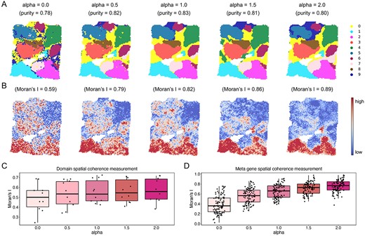
The illustrative analysis of flexible usage of spatial information on spatial domains and meta genes achieved by SpaSRL using the BC slice. (A) Spatial domains generated by SpaSRL under a variety of alpha settings. The identified spatial domains are distinguished using different colours and are shown on the spatial coordinates. The cluster purity is used to compare the similarity between the identified spatial domains and the ground truth annotations. (B) The spatial distribution of representative functional meta genes (focused on the bottom two spatial domains) identified by SpaSRL under a variety of alpha settings. Moran’s I measures the spatial autocorrelation of these functional meta genes. (C) Spatial coherence measurements of the identified domains from (A). (D) Spatial coherence measurements of the top 50 functional meta genes using Moran’s I statistics.
SpaSRL provides more biological insights into intratumour heterogeneity on breast cancer
We had demonstrated that SpaSRL can effectively dissect intratumour heterogeneity in BC as complementary to histopathological annotation (Figure 2C). In fact, SpaSRL can identify domain-specific functional genes (see Methods) and enhance the spatial expression patterns of individual genes, thus providing more insights to explore the molecular mechanisms underlying tumour heterogeneity.
In total, we obtained 357 spatial functional genes for all the identified domains (see Methods) (Supplementary Figure 13). These spatial functional genes show high-transcriptional specificity across spatial clusters and reveal distinct tumour microenvironments in the annotated cancer regions (Figure 4A). Then, performing cancer hallmark enrichment analysis (see Methods), we found that these spatial functional genes involved in different cancer-related biological processes, suggesting the potential cancer progression (i.e. surrounding tumour |$\to$| tumour |$\to$| invasive) in BC slice from the overall hallmark activation perspective (Figure 4B). These results indicated that SpaSRL could discover spatial functional genes with biological correspondence to heterogeneous tumour states.
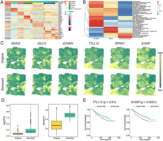
SpaSRL provides more biological insights into intratumour heterogeneity in BC sample. (A) The heatmap of original expression profiles of top five functional genes for each spatial domain identified by SpaSRL in Figure 2C. Each row of the heatmap indicates a gene and each column indicates a spot. The spots are labelled by histopathological annotations and SpaSRL assignments using column side colours. (B) The cancer hallmark enrichment of 357 functional genes in the Invasive, Tumour and Surrounding tumour regions. (C) Spatial expression of selected domain marker genes before (above) and after (below) data denoising. (D) The change of gene differential expression and spatial autocorrelation patterns before and after data denoising. FC: fold change of gene expression. (E) Survival analysis of the originally identified marker gene (i.e. TTLL2) and the newly identified marker gene (i.e. S100P).
In addition, we validated the effectiveness of SpaSRL on denoising expression profiles to enhance or recover gene spatial expression patterns. After SpaSRL denoising, some spatial functional gene expressions (e.g. IGHG2, IGHC3, JCHAIN, TTLL12, GFRA1 and S100P) appeared more spatially smoothed and with greater domain specificity on spots in situ (Figure 4C). The overall comparison of gene LFC and Moran’s I values quantifies the significant improvement of spatial expression coherence and biological specificity across domains brought by SpaSRL denoising (Wilcoxon signed-rank test |$P<{10}^{-16}$| for LFC and |$P<{10}^{-13}$| for Moran’s I, Figure 4D). We found 261 novel spatial functional genes in addition to the 96 genes that were ever identified in the original data under the same criteria (see Methods), indicating SpaSRL of potential to reveal new biological discoveries of disease. To further investigate this issue, we used two spatial domains (i.e. domain 0 in surrounding tumour region and domain 1 in invasive tumour region, Figure 2C) to display the LFCs of these spatial functional genes before and after denoising (Supplementary Figure 14) and observed the obvious enhancement of gene spatial expression for individual domains. Among the spatial functional genes for domain 1, 20 (out of 44) were validated to be the potential prognostic risk factors for breast cancer (Supplementary Table 1). These prognostic-related genes contained the originally and newly discovered genes. For example, TTLL12 is an originally identified gene and ever reported to be positively correlated with poor prognosis in breast cancer [35] (Figure 4E). S100P is a new-found gene and proved as involved in the aggressive properties of breast cancer cells [36], which is upregulated in breast cancer and associated with poor prognosis (Figure 4E). These findings indicate that SpaSRL can distinguish intratumour heterogeneous regions but also can provide the comprehensive biological insights into the underlying heterogeneity by combing data denoising and spatial functional genes identification.
SpaSRL identifies fine-grained mouse brain structures in 10× Visium datasets
We then applied SpaSRL to 10× Visium mouse brain sagittal sections (i.e. anterior and posterior samples) for comprehensive characterization of the fine-structured tissue architecture and region-specific functional genes. We took the haematoxylin and eosin (H&E) images of each dataset and the corresponding anatomical diagrams obtained from Allen Brain Atlas (ABA) [33] as reference, and compared the anatomical regions with computationally generated domains by SpaSRL and other competing methods.
For the anterior slice, SpaSRL distinguished the domains largely consistent with the ABA and H&E references, including the layered cortical structures of five cerebral cortex (CTX) domains (i.e. domains 1, 2, 5, 6 and 7) and fibre tract (i.e. domain 3), and a subtle region of the lateral ventricle (VL) section (i.e. domain 13), while other benchmarking methods failed to localize the fine structures or identified fewer sections (Figure 5A and Supplementary Figure 15). In addition, BayesSpace can also identify the layered domains (i.e. CTX and fibre tract), but SpaSRL’s separation showed better transcriptional specificity on the layer known marker genes (from outer to inner layers: Ptgds, Rasgrf2, Stx1a, Myl4, Nptx1 and Plp1) (Figure 5B and Supplementary Figure 16). For the VL section, SpaSRL also detects its specific functional meta gene (Figure 5C), where the top-weighed genes are Enpp2 and Ttr (Figure 5D), two marker genes of choroid plexus epithelial cell type which is enriched in VL region [37]. Thus, SpaSRL can detect the fine-grained brain structures and identify the biologically informative genes that underlie the corresponding spatial domains.
![SpaSRL identifies tissue structures and functional genes/meta genes in mouse brain sagittal anterior (n = 3696 spots) (A–D) and posterior (n = 3353 spots) (E–H) slices. The corresponding anatomical definitions obtained from the Allen Mouse Brain Atlas (First image in A and E) are shown as references. The identified spatial domains by all the involved approaches are illustrated on the spatial coordinates and distinguished using different colours without anatomical correspondence. Fine anatomical regions, for example CTX, fibre tract, VL sections in (A) and DG, CA sections in (E) are marked by red circles on reference images and computational results (if any exists). (B) The original expression heatmap of known marker genes separates the CTX and fibre tract layers identified by SpaSRL. SpaSRL CTX layers (from outer to inner) contain domains 6, 2, 7, 5 and 1; fibre tract is the domain 3. (C) The representative functional meta gene identified by SpaSRL to characterize VL section. (D) The original spatial expression of the top two-weighted functional genes in the representative functional meta gene from (C). (F) The representative meta gene identified by SpaSRL to characterize two separated DG sections. (G) Spatial expression of the two marker genes of DG sections before and after denoising. (H) The GO enrichment of the representative meta genes from (C). The size indicates the number of functional genes enriched in each GO term, and the colour indicates the statistical significance (adjusted by false discovery rate [FDR]) of enrichment in each GO term. The terms are grouped by GO subontology. BP, biological process; CC, cellular component; MF, molecular function.](https://oup.silverchair-cdn.com/oup/backfile/Content_public/Journal/bib/24/4/10.1093_bib_bbad197/1/m_bbad197f5.jpeg?Expires=1749148191&Signature=l2-7LV16-x4EQZljO9q1uOgo3w0oEj6UB4Fy9HRhoY-fDVyxp3xn2IEJ9Bb4sey~r17ax4XDgRKUxon~oi4GOBI3SXgG6ThYWe3MBgSKVJKsOstnC2qEtx3uPSn3D6TDZui6UYlgsuRm5UFq7FY4dzm1FRDkt1Waiggxq5FG-F-5X~TmsYNq6Pll-6U7PGuoMPYqU0H7dLPIEWFnV9~BI3DRxjlNW9DRwxz3EGnqThp2fYGfkwfZMnisvdpkeaYHkm84RH6hNnxdYLycKDB7mZiLYNraaorAsYtehTafBA1OrwZigOSvu7KYwTJscipDnn2mMSYpT1nbsVYRrzKh~A__&Key-Pair-Id=APKAIE5G5CRDK6RD3PGA)
SpaSRL identifies tissue structures and functional genes/meta genes in mouse brain sagittal anterior (n = 3696 spots) (A–D) and posterior (n = 3353 spots) (E–H) slices. The corresponding anatomical definitions obtained from the Allen Mouse Brain Atlas (First image in A and E) are shown as references. The identified spatial domains by all the involved approaches are illustrated on the spatial coordinates and distinguished using different colours without anatomical correspondence. Fine anatomical regions, for example CTX, fibre tract, VL sections in (A) and DG, CA sections in (E) are marked by red circles on reference images and computational results (if any exists). (B) The original expression heatmap of known marker genes separates the CTX and fibre tract layers identified by SpaSRL. SpaSRL CTX layers (from outer to inner) contain domains 6, 2, 7, 5 and 1; fibre tract is the domain 3. (C) The representative functional meta gene identified by SpaSRL to characterize VL section. (D) The original spatial expression of the top two-weighted functional genes in the representative functional meta gene from (C). (F) The representative meta gene identified by SpaSRL to characterize two separated DG sections. (G) Spatial expression of the two marker genes of DG sections before and after denoising. (H) The GO enrichment of the representative meta genes from (C). The size indicates the number of functional genes enriched in each GO term, and the colour indicates the statistical significance (adjusted by false discovery rate [FDR]) of enrichment in each GO term. The terms are grouped by GO subontology. BP, biological process; CC, cellular component; MF, molecular function.
For the posterior slice, only SpaSRL recognized the dentate gyrus (DG) (i.e. domain 14), and cornu ammonis (CA) (i.e. domain 12) sections of the hippocampus region, just as the H&E-stained shape on original image and ABA reference (Figure 5E and Supplementary Figure 17). On the slice, the domain 14 contains two separated regions that can be clearly highlighted by the SpaSRL obtained meta gene (Figure 5F) and two DG marker genes (i.e. Prox1 [38] and C1ql2 [39]). Moreover, SpaSRL greatly improved the marker gene spatial expression and specificity on the denoised profiles (Figure 5G). We then extracted the spatial functional genes of this domain and performed functional enrichment analysis (see Methods) (Supplementary Figure 18). We found these genes were enriched in many biological functions related to hippocampus DG region e.g. neurogenesis, generation of neurons and nervous system development [40] (Figure 5H). These results indicate that SpaSRL not only can detect subtle spatial biological signals but also can effectively decode spatial expression patterns from spot and gene perspectives with correspondent associations and biological interpretations.
SpaSRL reveals spatial expression landscape in slide-seqV2 mouse olfactory bulb dataset
Next, we used the mouse olfactory bulb Slide-seqV2 dataset to illustrate the scalability of SpaSRL on high-resolution spatial domain and functional gene identification. This serves as an in-depth supplement to the benchmarking instances on multiple high-resolution platforms (Supplementary Figures 8–10). For better illustration, we also took the ABA anatomical diagram as reference and compared SpaSRL with other spatial domain detection methods (e.g. Vesalius, SEDR, SpaGCN, STAGATE and SpatialPCA) (Figure 6A and Supplementary Figures 19–23).
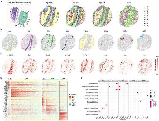
SpaSRL reveals spatial expression landscape in Slide-seqV2 olfactory bulb data (n = 21 724 spots). (A) The regional structure diagrams from ABA and spatial domains identified by SpaSRL, Vesalius, SpaGCN and SEDR. The Allen reference is used for illustrating the clustering results. Clustering outcomes of STAGATE and SpatialPCA are in Supplementary Figures 19 and 22. Individual loadings of each spatial domain identified by SpaSRL (B) and the expression of corresponding marker genes (C). Domain individual loadings from competing methods are illustrated in Supplementary Figures 19-23. (D) The original expression heatmap of the top 40 functional genes identified by SpaSRL. Gene expression is scaled through z-score normalization across spots. (E) The bubble plot of GO BP enrichment results of all the functional genes for the involved domains. The dot size indicates the number of functional genes enriched in each GO term and the colour indicates the FDR-adjusted significance of enrichment in each GO term.
According to the diagram, the mouse olfactory bulb exhibits architecture of multiple layers, while SpaSRL can delineate the layered domains of clear boundaries that are highly consistent with the reference structure (Figure 6A). From outer to inner, we then labelled each SpaSRL’s domain as olfactory nerve layer (ONL, domain 3), glomerular layer (GL, domains 2 and 4), external plexiform layer (EPL, domain 1), mitral cell layer (MCL, domain 8), granule cell layer (GCL, domain 0), rostral migratory stream (RMS, domain 5), granular layer of accessory olfactory bulb (AOBgr, domain 6) and accessory olfactory bulb (AOB, domain 7) (Figure 6B). Moreover, our obtained domains show good alignment with known marker expressions (Figure 6C). For example, the ONL region was revealed by the high expression of S100a5, which is restrictedly stained in this area as confirmed in previous experiments [41]. The GL and EPL are two adjacent layers that can be defined by the combined markers e.g. Cck and Doc2g, which were previously used in Ståhl et al.’s work [2]. The MCL structure, a thin morphological layer [42], was characterized by the presence of gene Shisa3 [2]. The GCL layer can be clearly separated by the abundance of the known neuron marker Pcp4 [43]. As for the inner three regions i.e. RMS, AOBgr and AOB, specific signatures (i.e. Mbp for RMS [44], Tac1 for AOBgr [33] and Fxyd6 for AOB [45]) were enriched in respective regions, consistent with independent findings or experiments. Collectively, these results further illustrated the ability of SpaSRL to reveal the fine-grained tissue structures from high-resolution SRT datasets (Figure 6A–C and Supplementary Figures 8–10).
In addition, SpaSRL identifies the spatial functional (meta) genes of multiple domains (see methods), which can obviously reveal the transcriptional differences across layered architecture (Figure 6D and Supplementary Figure 24). We further made functional enrichment analysis of these genes to explore the possible biological processes underlying different regions (Figure 6E). We observed that the gene sets for RMS are enriched in regulation of neurogenesis and glial cell differentiation, in accord with the fact that RMS is abundant of neuron precursors and glial cells as a region responsible for neuroblast migration [44]. The GCL, MCL and EPL regions were marked by processes associated with nerve signals transmission e.g. (trans-) synaptic signalling, chemical synaptic transmission or electron transport chain. The results are consistent with the biological facts that these layers have many types of neuron cells (e.g. mitral cells in MCL, granule cells in GCL) which receive and transmit the olfactory signals through synaptic connections [46]. As for the ONL region which resides in the nasal epithelium, the identified gene sets show the potential epithelial process (i.e. epithelial cell proliferation) in addition to its neuron function [46]. These results suggest good biological coherence between our functional (meta) genes and spatial domains. Thus, we can see, for higher resolution SRT data, SpaSRL is capable to effectively unveil the spatially organizational expression landscape from domain and metagene perspectives.
DISCUSSION
Spatial mRNA measurements provide new perspectives to define biological heterogeneities of tissues and diseases under spatial context. The fundamental issue of deciphering tissue heterogeneity is to accurately capture the relationship between spots and the functional genes with spatial coherence and co-expression. However, the current methods still focus on the individual task and there is a great challenge to join the two tasks into a unified model while flexibly incorporating spatial information. In this work, SpaSRL was designed as such a scalable framework that accounts for these requirements. SpaSRL provides a computationally efficient tool to obtain the spot–spot relations and the functional genes with flexibly spatial correlation constraint, which are then used for accurate downstream analysis, including spatial domain detection, spatial functional genes/meta genes identification and data denoising. The superiority of SpaSRL not only is reflected on the accurate identification of spatial domains and functional genes on multiple datasets of various technologies i.e. 10× Visium, Slide-seqV2, but also can control the usage of spatial information to impact the identification of spatial domain and functional genes. In particular, the application on breast slices and brain slices demonstrated that SpaSRL reveals the tissue structures and the corresponding spatial functional genes for interpreting tissue heterogeneity, suggesting that SpaSRL is more suitable for deciphering complex spatial expression landscape in SRT study.
The effective usage of spatial information is key to the superiority of SpaSRL in SRT study. Specifically, SpaSRL first uses spatial information to enhance the shared information between neighbouring spots. Then, SpaSRL builds a novel self-representation model to decode the shared expression between spots from the enhanced data of the low-dimensional space and the original space. The stepwise approaches of SpaSRL take spatial information as a soft constraint to impact the spatial coherence of the spatial domain and functional meta genes and to mitigate SRT data noise or bias. In addition, the novel self-representation learning model achieves dimension reduction and spatial domain detection into a unified model. This approach allows the spatially aware strategy of SpaSRL to transfer spatial correlation constraints between the two tasks. Thus, compared with the current methods, SpaSRL not only flexibly controls the usage of spatial information but also improves the identification of biologically informative spatial domain and functional genes by leveraging spatial information.
Although SpaSRL provides the joint analysis of the spatial domain detection and the functional genes identification, SpaSRL still performs the individual gene analysis and cannot track which functional gene network module contributes to each spatial domain, which is a limitation of SpaSRL for application to the in-depth analysis of biological interpretations. Certainly, most methods are compromised to use a separate manner: first to detect spatial domain and subsequently to infer gene networks (or vice versa). However, the splitting solution may cause untraceable biological variabilities, even leading to biased outcomes. Therefore, further study of the joint analysis of domains and gene networks under spatial context is warranted.
SpaSRL is a spatially aware self-representation learning method that unify the identification of spatial domains and functional (meta-) genes, relying on a joint model to optimally transfer spatial correlation constraint between the two tasks.
SpaSRL provides a novel tunable strategy to achieve the flexible integration of spatial information via an enhancing-decoding schema as complementary to the current usage of spatial information.
SpaSRL is a user-friendly and computationally efficient Python tool that can be scalable for diverse SRT platforms.
ACKNOWLEDGEMENTS
We thank the anonymous reviewers for useful suggestions.
FUNDING
This work is supported by National Natural Science Foundation of China (Grant No. 62202120) and the R&D project of Pazhou Lab (Huangpu) under Grant 2023 K0602.
AUTHORS’ CONTRIBUTIONS
Q.S. and C.Z conceived and designed the framework and the experiments. L.W. and L.X. performed the experiments. L.W. and W.H. developed the Python package and documentation website of the framework. L.W., Q.S. and C.Z analysed the data and wrote the paper. Q.S. and C.Z revised the manuscript.
DATA AVAILABILITY
The human dorsolateral prefrontal cortex (DLPFC) datasets are available in the spatialLIBD package (http://spatial.libd.org/spatialLIBD). The Mouse Brain Sagittal, Invasive Ductal Carcinoma and Human Breast Cancer datasets are available at 10x Genomics website (https://www.10xgenomics.com/resources/datasets). The Slide-seqV2 data is available at https://singlecell.broadinstitute.org/single_cell/study/SCP815. The STARmap dataset is available at https://www.starmapresources.com/data. The osmFISH dataset is available at https://github.com/drieslab/spatial-datasets.
CODE AVAILABILITY
Python source code of SpaSRL, under the open-source BSD 3-Clause license, is available at https://github.com/zccqq/SpaSRL. The documentation website provides the installation guide, tutorials and API references, which is available at https://spasrl.readthedocs.io/. SpaSRL is also published as a Python package named ‘spasrl’ on Python Package Index (PyPI) at https://pypi.org/project/spasrl/ and can be directly installed via the pip installer.
Author Biographies
Chuanchao Zhang received the PHD from Wuhan University, Wuhan, China, in 2017. He is currently an assistant research fellow in Key Laboratory of Systems Health Science of Zhejiang Province, Hangzhou Institute for Advanced Study, University of Chinese Academy of Sciences, Chinese Academy of Sciences, Hangzhou 310024, China. His current research interests include machine learning, deep learning, single-cell transcriptomics and spatial transcriptomics.
Xinxing Li is a master student in College of Informatics, Huazhong Agricultural University, Wuhan, China. Her current research interests include single-cell transcriptomics and spatial transcriptomics.
Wendong Huang is a master student in College of Informatics, Huazhong Agricultural University, Wuhan, China. His current research interests include single-cell transcriptomics and spatial transcriptomics.
Lequn Wang is pursuing his PhD degree in the Center for Excellence in Molecular Cell Science. His current research interests include bioinformatics, machine learning, single-cell multi-omics and spatial transcriptomics.
Qianqian Shi received the PHD from Shanghai Institute of Biological Sciences, University of Chinese Academy of Sciences, Chinese Academy of Sciences, China, in 2017. She is currently an associate professor at College of Informatics, Huazhong Agricultural University, Wuhan, China. Her current research interests include machine learning, deep learning, network biology, computational biology, single-cell transcriptomics and spatial transcriptomics.
