


Abstract
Determining intrinsically disordered regions of proteins is essential for elucidating protein biological functions and the mechanisms of their associated diseases. As the gap between the number of experimentally determined protein structures and the number of protein sequences continues to grow exponentially, there is a need for developing an accurate and computationally efficient disorder predictor. However, current single-sequence-based methods are of low accuracy, while evolutionary profile-based methods are computationally intensive. Here, we proposed a fast and accurate protein disorder predictor LMDisorder that employed embedding generated by unsupervised pretrained language models as features. We showed that LMDisorder performs best in all single-sequence-based methods and is comparable or better than another language-model-based technique in four independent test sets, respectively. Furthermore, LMDisorder showed equivalent or even better performance than the state-of-the-art profile-based technique SPOT-Disorder2. In addition, the high computation efficiency of LMDisorder enabled proteome-scale analysis of human, showing that proteins with high predicted disorder content were associated with specific biological functions. The datasets, the source codes, and the trained model are available at https://github.com/biomed-AI/LMDisorder.
Introduction
Proteins were thought to have a stable tertiary structure when performing their functions. However, Romero et al. [1] suggested that about 15 000 proteins or long protein regions in SwissProt [2] do not have a well-defined 3D structure. These intrinsically disordered proteins or protein regions (IDPs/IDRs) enriched our understanding of the sequence-structure–function relation of proteins. For example, lacking a rigid structure, IDPs/IDRs can transform between a group of transient and mutually transforming structural states [3]. Some functions directly require structural flexibility such as linkers between structured domains whereas other IDPs can undergo disorder-to-order transitions when interacting with specific bioactive molecules and serve as specific chaperones for certain proteins. These binding regions or molecular recognition features were found in modular proteins participating in signaling and regulation [4, 5]. The plasticity and flexibility of these functional modules, allow IDPs/IDRs to adopt varying conformations to interact with different partners in signal transmission, assembly and regulation, resulting in their involvement in many human diseases, including cardiovascular disease, cancer, various genetic diseases and neurodegenerative diseases [6]. Multi-structure states of IDPs [3, 7] may be evolutionarily advantageous, as suggested by higher degree of intrinsic disorder in natural proteins than in random sequences [8]. Thus, identifying IDPs/IDRs is crucial to comprehend and resolve the causes and impacts of these unstructured states [9].
Several experimental techniques have been employed to identify IDPs/IDRs including X-ray crystallography, nuclear magnetic resonance (NMR) and circular dichroism (CD) [7, 10]. However, due to the high-cost, laborious and time-consuming nature of these experiments, computational tools for predicting IDRs/IDPs in protein sequences have been an active area of research for the past 20 years.
IDP prediction was initially based on small-scale machine learning models [11], using neural networks and support vector machines. As more data and powerful tools emerged, the deep learning models have come to the forefront, in methods such as ESpritz [12], SPOT-Disorder [13], NetSurfP-2.0 [14], AUCpreD [15], SPINE-D [16] and SPOT-Disorder2 [17]. Depending on the input, these methods for protein disorder prediction can be divided into two categories: single-sequence and sequence profile from multiple sequence alignment. The single-sequence-based methods leverage the composition and connectivity of the single protein sequence along with its derived information such as statistical potentials and amino acid propensities [18–20]. These methods allow fast computation but are less accurate than those using evolutionary sequence profiles [21, 22] because sequence conservations are important indicators for structure and function. Examples of profile-based methods are SPINE-D [16], MDFp2 [23], AUCpreD [15], SPOT-Disorder [13] and SPOT-Disorder2 [17]. However, the exponential increase in the library size of protein sequences makes profile generation computationally more and more intensive. Moreover, most proteins (>90%) do not pertain to large sequence clusters [24] and, as a result, their sequence profiles may not be that useful.
Recently, the unsupervised pretrained language models have been applied to extract features from protein sequences [25–28], which has shown very promising results in the downstream forecast, such as tertiary contact, ontology-based protein function, secondary structure, contact map and mutational effect [28–33]. These breakthroughs inspire us to exploit the language models for disorder prediction. A recent study [30] evaluated and discussed the performance of different models for protein representation, indicating that ProtTrans achieved the best performance in most of the tasks. However, ProtTrans has not yet been used for protein disorder prediction. In this work, we employed ProtTrans language model to predict the intrinsic disorder regions of protein.
Here, we present LMDisorder, an alignment-free sequence-based prediction of protein intrinsic disorder. Using a recently released pretrained language model [34], LMDisorder can generate informative sequence representations fast and make an accurate prediction. Specifically, we first leveraged the pretrained language model ProtTrans to produce the sequence embedding. Then, transformer networks were employed to capture the sequence patterns including long-range dependencies between the residues, followed by a fully connected layer for predicting protein disorder probabilities. LMDisorder was shown to be superior to or as good as other profile-based methods including SPOT-Disorder2 on different datasets with its computational efficiency as efficient as single-sequence-based techniques. The high computation efficiency of LMDisorder enabled proteome-scale analysis of human, showing that proteins with high predicted disorder content were associated with specific biological functions.
MATERIALS AND METHODS
Datasets
In our experiments, the datasets were obtained from previous studies [17, 34], as shown in Table 1. Briefly, we obtained 4229 protein sequences (DM4229), which contain 72 fully disordered chains from DisProt v5.0 [35] and 4157 high-resolution X-ray crystallography structures from PDB (prior to the 5 August 2003). These proteins were randomly divided into a training set (2700 proteins), a validation set (300 proteins) and a Testing set (1229 proteins, DM1229). According to BLASTClust [36], the sequence similarity of these proteins is <25%. Furthermore, we also employed four independent test datasets SL329, DisProt228, Mobi9230 and DisProt452. The SL329 dataset is selected from the SL477 protein set, which is released by Sirota et al. [37]. The overlap between DM4229 and SL477 was removed to obtain an independent test set containing 329 non-redundant sequences (SL329). DisProt228 is the subset from DisProt Complement [22] and consists of the proteins in DisProt database v7.0. Mobi9230 was obtained from MobiDB [38] with experimental annotation, which derived from manually curated database and primary data (e.g., from PDB structures). We constructed a novel dataset DisProt452, which consists of the proteins deposited to the DisProt database from June 2020 to December 2022. After removing the long proteins (>700 residues) and the homologous proteins in our training set and validation set (25% sequence identity cutoff with BLASTClust [36]), we obtained 452 proteins and built a novel independent test dataset DisProt452. Meanwhile, we respectively created the subsets of SL329 and DM1229, named SL250 and Test1185, all of which are the same datasets employed previously by SPOT-Disorder and SPOT-Disorder2 [17]. In Table 1, We have detailed the number of proteins, ordered and disordered residues as well as the percentage of disorder in each dataset. These independent test datasets contain the latest data, such as the newly annotated proteins in DisProt452, which were deposited to the DisProt database from June 2020 to December 2022.
The number of proteins, ordered and disordered residues as well as the percentage of disorder in each dataset
| Dataset | No. of proteins | No. of ordered residues | No. of disordered residues | Percentage of disorder |
|---|---|---|---|---|
| Validation | 300 | 61 231 | 6083 | 9.04% |
| DM1229 | 1229 | 276 748 | 29 082 | 9.51% |
| SL329 | 329 | 51 292 | 39 544 | 43.53% |
| DisProt228 | 228 | 30 772 | 18 811 | 37.94% |
| Test1185 | 1185 | 246 616 | 26 515 | 9.71% |
| SL250 | 250 | 32 261 | 21 173 | 39.62% |
| Mobi9230 | 9230 | 2 011 126 | 828 642 | 29.18% |
Protein sequence features
Language model representation. LMDisorder utilizes the recent protein language model ProtT5-XL-U50 [34] (denoted as ProtTrans) for feature extraction. This is a transformer-based auto-encoder named T5 [39], which was pretrained in a self-supervised manner on UniRef50 [40], learning to predict masked amino acids. We extracted the hidden states from the last layer of the ProtTrans encoder as sequence features, which is an |$n\times 1024$| matrix (|$n$| is the sequence length). We have also examined another pretrained model, ESM-1b [29] (denoted as ESM), which was also pretrained on UniRef50 with transformer. Sequence features by ESM are an |$n\times 1280$| matrix. The computational costs of inference for both ProtTrans and ESM are low, and the feature extraction process of our whole benchmark datasets (~4800 sequences) can be completed within 10 minutes on an Nvidia GeForce RTX 3090 GPU.
Evolutionary information (for ablation study). We have also tested evolutionary-derived features (position-specific scoring matrix, PSSM and hidden Markov models, HMM) for feature ablation studies. PSSM was obtained by performing PSI-BLAST [36] search against UniRef90 [40] with three iterations and an E-value of 0.001. HHblits was employed to generate HMM profile [41] by aligning a query sequence against UniClust30 [42] with default parameters. Each residue was encoded into a 20-dimensional feature vector in PSSM and HMM.
Predicted structural properties (for ablation study). Putative structural properties were generated by utilizing SPIDER3 [43], whose inputs include protein sequence, PSSM profiles and HMM profiles. We extracted four types of structural features from the outputs of SPIDER3: (1) Solvent accessible surface area. (2) The sine and cosine values of the four protein backbone torsion angles (θ, ϕ, ψ and τ). (3) Half sphere exposures, which are the numbers of spatially neighboring residues in the top and bottom half of the contacting sphere: the boundary of the two hemispheres was determined by the Cα-Cα and Cα-Cβ direction vectors. (4) Predicted probabilities of the three secondary structures (α-helix, β-sheet and random coil). Each residue was encoded into a 14-dimensional vector using SPIDER3. Values in PSSM, HMM and SPIDER were further normalized to scores between 0 to 1 using the min–max normalization:
where v is the original feature value, and Min and Max are the smallest and biggest values of this feature type observed in the training set.
The architecture of LMDisorder
The overall architecture of LMDisorder is shown in Figure 1. First, the protein sequence is inputted into the pretrained language model ProtTrans to yield the sequence embedding, which is augmented by Gaussian noise to avoid overfitting. Then, the transformer networks are employed to capture the sequence patterns including long-range dependencies between the residues. This is followed by a fully connected layer adopted to predict protein disorder probabilities.

The architecture of LMDisorder. A protein sequence is input into ProtTrans to produce the sequence embedding. The embedding is augmented by Gaussian noise and further encoded through the transformer networks to capture the long-range sequence patterns. The encoded representation is input to a fully connected layer for predicting disorder probabilities.
Transformer networks
We stack N identical transformer [44] layers to learn the sequence representations. Each transformer layer has two sub-layers, a multi-head self-attention module, and a position-wise feed-forward network. A residual connection [45] is employed around each of the two sub-layers, followed by the layer normalization [46]. Let |$\boldsymbol{H}\in{\mathbb{R}}^{n\times d}$| denotes the input of the self-attention module, where n is the sequence length and d is the hidden dimension. The input of the |${l}^{\text{th}}$| layer |$\boldsymbol{{H}}^{(l)}$| is projected by three matrices |$\boldsymbol{W}_Q\in{\mathbb{R}}^{d\times{d}_K}$|, |$\boldsymbol{W}_K\in{\mathbb{R}}^{d\times{d}_K}$| and |$\boldsymbol{W}_V\in{\mathbb{R}}^{d\times{d}_V}$| to get the corresponding query, key, and value representations |$\boldsymbol{Q},\boldsymbol{K},\boldsymbol{V}$| as below:
The scaled dot-product self-attention is then calculated according to the following equation:
where |$\sqrt{d_K}$| is a scaling factor and |$\boldsymbol{A}$| is a matrix capturing the similarities between queries and keys. Instead of performing a single attention function, multi-head attention was employed to jointly attend to information from different representation subspaces at different positions. We linearly projected the queries, keys and values h times, perform the attention function in parallel, and finally concatenate them together. In this work, |${d}_K={d}_V=d/h$|.
Fully connected layer and noise augmentation
The output of the last transformer layer is input to a fully connected layer to predict the protein disorder probabilities for all n amino acid residues of the protein:
where |$\boldsymbol{H}^{\left(N+1\right)}\in{\mathbb{R}}^{n\times d}$| is the output of the |${N}^{\text{th}}$| transformer layer; |$\boldsymbol{W}\in{\mathbb{R}}^{d\times 1}$| is a learnable weight matrix; |$b\in \mathbb{R}$| is a bias term, and |$\boldsymbol{Y}^{\prime}\in{\mathbb{R}}^{n\times 1}$| is the predictions for the n residues. The sigmoid function normalizes the output of the fully connected layer into binding probabilities from 0 to 1. In addition, to avoid overfitting, the sequence features from ProtTrans are augmented by Gaussian noise before being fed to the transformer networks while training:
where |$\boldsymbol{H}^{(0)}$| is the sequence features from ProtTrans, |$\boldsymbol{X}$| is a matrix of random values from the standard normal distribution with the same size as |$\boldsymbol{H}^{(0)}$|, and ε is a hyperparameter to regulate the augmentation.
Implementation details
We utilized the training set to train LMDisorder, and the validation set to evaluate its generalization on unseen proteins. The training process lasted at most 50 epochs and we chose the model in the epoch with the best performance on the validation set as the final model. The validation performance was optimized by choosing the best feature combination and searching all hyperparameters through a grid search. Specifically, we employed a 2-layer transformer network with 128 hidden units and the following set of hyperparameters: h = 4, ε = 0.05, and a batch size of 12. The dropout rate was set to 0.3 to avoid overfitting. We utilized the Adam optimizer [47] with a learning rate of 3 × 10⁻⁴ for model optimization on the binary cross-entropy loss. We implemented the proposed model with Pytorch 1.7.1 [48].
Evaluation metrics
Similar to previous studies [17, 34], we employed the area under the receiver operating characteristic curve (|${\text{AUC}}_{\text{ROC}}$|), precision (Pr), sensitivity (Se), specificity (Sp), the area under the precision-recall curve (|${\text{AUC}}_{\text{PR}}$|), Matthews correlation coefficient (MCC), and the weighted score Sw (Sw = sensitivity + specificity – 1) to evaluate the performance of the method developed:
where TN, TP, FN and FP denote true negatives, true positives, false negatives and false positives, respectively.
RESULTS AND DISCUSSIONS
Feature importance and ablation analysis
The results of LMDisorder on the validation set and two independent test sets are shown in Table 2. It can be seen that the fractions of disordered residues are very different in different datasets. The fraction of disordered residues is only 9.0% of all residues in the validation set, compared to 9.5% in DM1229 and 56.5% in SL329. As |${\text{AUC}}_{\text{ROC}}$| is a balanced metric, similar performance for two data sets differed significantly in disorder content, indicates the robustness of our method. The |${\text{AUC}}_{\text{ROC}}$| of LMDisorder on validation set and DM1229 datasets are 0.940 and 0.920, and the |${\text{AUC}}_{\text{PR}}$| are 0.732 and 0.705, respectively. Although the disordered residues dominate the SL329 set, LMDisorder still achieved a similar performance with an |${\text{AUC}}_{\text{ROC}}$| of 0.911 and |${\text{AUC}}_{\text{PR}}$| of 0.909, respectively.
The performance of LMDisorder on the validation and two independent test sets according to various measures, including AUCROC, AUCPR, MCC, Pr, Se, Sp, along with the statistics of the number of disordered and ordered residues
| Dataset | |${\text{AUC}}_{\text{ROC}}$| | |${\text{AUC}}_{\text{PR}}$| | MCC | Pr | Se | Sp | # Order | # Disord |
|---|---|---|---|---|---|---|---|---|
| Validation | 0.940 | 0.732 | 0.646 | 0.746 | 0.598 | 0.980 | 61 231 | 6083 |
| DM1229 | 0.920 | 0.705 | 0.621 | 0.756 | 0.560 | 0.981 | 276 748 | 29 082 |
| SL329 | 0.911 | 0.909 | 0.655 | 0.947 | 0.625 | 0.973 | 51 292 | 39 544 |
To examine the importance of various features for disorder prediction, we performed feature ablation experiments. As shown in Figure 2 and Supplementary Table S1, the model with either ProtTrans or ESM language model as sequence features performs significantly better than the profile-based models including PSSM+HMM and PSSM+HMM + SPIDER. Among them, the |${\text{AUC}}_{\text{ROC}}$| of the model using ProtTrans on validation set, DM1229 and SL250 are 0.940, 0.920 and 0.905, respectively, which is better than the model using ESM (0.922, 0.912 and 0.885). By comparison, the models using PSSM+HMM and PSSM+HMM + SPIDER features yield |${\text{AUC}}_{\text{ROC}}$| values of only 0.847, 0.840, 0.806 and 0.893, 0.886, 0.855, respectively. We noted that combining ProtTrans and PSSM+HMM + SPIDER features did not improve the model, with the |${\text{AUC}}_{\text{ROC}}$| value of 0.938, 0.918 and 0.905 for the validation set, DM1229 and SL250 sets, respectively, indicating that the pretrained model ProtTrans may have captured the evolution information and structure information of proteins. Furthermore, we found that combining ProtTrans with ESM only led to minor changes. The |${\text{AUC}}_{\text{ROC}}$| on the three datasets was 0.936, 0.922 and 0.906, respectively. Furthermore, to examine the effect of Gaussian noise, we tested the model without Gaussian noise. As shown in Supplementary Table S1, when we removed Gaussian noise, the |${\text{AUC}}_{\text{ROC}}$| and |${\text{AUC}}_{\text{PR}}$| were 0.917 and 0.692, decreasing by 2.4 and 5.5%, respectively. These results demonstrated the usefulness of Gaussian noise.
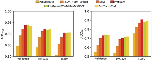
Comparison of different feature combinations as labeled on the Validation and two independent test sets (DM1229 and SL250). Method performance is measured by Area under ROC and PR curves (AUCROC and AUCPR).
Comparison with single-sequence-based methods
We compared LMDisorder with seven single-sequence-based methods (ESpritz-N, ESpritz-D, ESpritz-X, IUPred2A-short [49], IUPred2A-long and Spot-Disorder-Single [34]) on DM1229 and SL329. In addition, we compared to NetSurfP-3.0 [50], which is based on ESM-1b language model. The single-sequence-based methods employ sequence-derived features such as one-hot features. In this work, we obtained abundant protein representation from ProtTrans language model, which is found here effective for protein disorder prediction. Figure 3 compared the ROC curves and Supplementary Figure S1 and S2 compared the precision–recall curves produced by these methods on DM1229 and SL329, respectively, along with performance indicators listed in Table 3. Among all the methods compared, LMDisorder achieved the highest |${\text{AUC}}_{\text{ROC}}$| and MCC values in both datasets, while NetSurfP-3.0 achieved the second best. LMDisorder achieved the best results on SL329, with |${\text{AUC}}_{\text{ROC}}$| of 0.911, AUCPR of 0.910 and MCC of 0.655, which is 1.0% (|${\text{AUC}}_{\text{ROC}}$|), 1.4% (AUCPR) and 5.5% (MCC) higher than NetSurfP-3.0, respectively. LMDisorder and NetSurfP-3.0 achieved a comparable level on DM1229, where the |${\text{AUC}}_{\text{ROC}}$|, AUCPR and MCC of LMDisorder are 0.920, 0.705 and 0.621 respectively and the same indicators of NetSurfP-3.0 are 0.918, 0.732 and 0.620. It is worth noting that SPOT-Disorder-Single achieved the third best results on two datasets. For DM1229 dataset, the |${\text{AUC}}_{\text{ROC}}$|, AUCPR and MCC of SPOT-Disorder-Single are 0.868, 0.599 and 0.518, which are 5.6% (|${\text{AUC}}_{\text{ROC}}$|), 15% (AUCPR) and 17% (MCC) lower than LMDisorder, respectively. And on SL329, the |${\text{AUC}}_{\text{ROC}}$|, AUCPR and MCC of SPOT-Disorder-Single are 2.6% (|${\text{AUC}}_{\text{ROC}}$|), 2.6% (AUCPR) and 7.8% (MCC) lower than LMDisorder, respectively. For a more comprehensive comparison, we compared LMDisorder with other single-sequence-based methods on Mobi9230, and found our model consistently performed the best (Supplementary Table S3). The |${\text{AUC}}_{\text{ROC}}$| and AUCPR of LMDisorder are 0.863 and 0.8 respectively, while the second best method (NetSurfP-3.0) are 0.846 (|${\text{AUC}}_{\text{ROC}})$| and 0.8 (AUCPR). Additionally, we constructed a novel independent dataset DisProt452 and tested LMDisorder with other methods in Supplementary Table S4. The results have shown that LMDisorder still has the best performance. The |${\text{AUC}}_{\text{ROC}}$| and AUCPR of LMDisorder are 0.875 and 0.854, respectively, while the second best method (spot-disorder-single) are 0.840 (|${\text{AUC}}_{\text{ROC}}$|) and 0.817 (AUCPR). The consistent performance on multiple data sets further confirmed the robustness of our model.
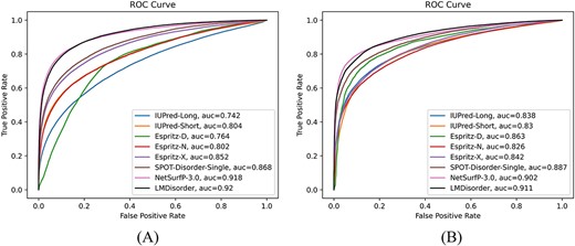
The receiver operating characteristic curves given by LMDisorder and other single-sequence-based methods on the (a) DM1229 and (b) SL329 sets.
The performance comparison of LMDisorder with several single-sequence-based methods on independent test sets DM1229 and SL329 according to AUCROC, AUCPR, MCC, Pr, Se and Sp. Bold fonts indicate the best results
| Dataset | Method | |${\text{AUC}}_{\text{ROC}}$| | |${\text{AUC}}_{\text{PR}}$| | MCC | Pr | Se | Sp |
|---|---|---|---|---|---|---|---|
| DM1229 | ESpritz-X | 0.852 | 0.565 | 0.503 | 0.640 | 0.459 | 0.973 |
| ESpritz-N | 0.802 | 0.480 | 0.431 | 0.619 | 0.358 | 0.977 | |
| ESpritz-D | 0.764 | 0.238 | 0.277 | 0.240 | 0.557 | 0.814 | |
| IUPred2A-short | 0.804 | 0.475 | 0.439 | 0.578 | 0.403 | 0.969 | |
| IUPred2A-long | 0.742 | 0.372 | 0.321 | 0.542 | 0.243 | 0.978 | |
| Spot-Disorder-Single | 0.868 | 0.599 | 0.518 | 0.707 | 0.432 | 0.981 | |
| NetSurfP-3.0 | 0.918 | 0.732 | 0.620 | 0.704 | 0.644 | 0.971 | |
| LMDisorder | 0.920 | 0.705 | 0.621 | 0.756 | 0.560 | 0.981 | |
| SL329 | ESpritz-X | 0.842 | 0.831 | 0.543 | 0.843 | 0.588 | 0.916 |
| ESpritz-N | 0.826 | 0.816 | 0.473 | 0.809 | 0.613 | 0.889 | |
| ESpritz-D | 0.863 | 0.829 | 0.608 | 0.873 | 0.620 | 0.931 | |
| IUPred2A-short | 0.830 | 0.811 | 0.506 | 0.799 | 0.649 | 0.874 | |
| IUPred2A-long | 0.838 | 0.833 | 0.552 | 0.812 | 0.648 | 0.884 | |
| Spot-Disorder-Single | 0.887 | 0.886 | 0.604 | 0.939 | 0.563 | 0.972 | |
| NetSurfP-3.0 | 0.902 | 0.897 | 0.621 | 0.864 | 0.773 | 0.912 | |
| LMDisorder | 0.911 | 0.910 | 0.655 | 0.947 | 0.625 | 0.973 |
Comparison with state-of-the-art profile-based methods
We compared LMDisorder with 12 profile-based methods [51] for DisProt228, including s2D [34], AUCpreD, JRONN [52], ESpritz-D, MFDp2 [53], DISOPRED [54], MobiDB-lite [55], ESpritz-N, SPINE-D, MFDp [23], SPOT-Disorder and SPOT-Disorder2. Among these, SPOT-Disorder2 is a state-of-the-art profile-based method, which had the best performance in CAID prediction [56]. The profile-based methods [16, 17] usually use the evolutionary sequence profiles obtained from multiple sequence alignment [21, 22] created mostly from HHBlits [41] and PSI-Blast [36]. In general, profile-based methods are more accurate than single-sequence-based, although these methods will take more time to calculate the features. As shown in Table 4, LMDisorder improved over 11 Profile-based methods, while achieving similar performance as SPOT-Disorder2. The |${\text{AUC}}_{\text{ROC}}$|, |${\text{AUC}}_{\text{PR}}$|, MCC and Sw of LMDisorder are 0.800, 0.700, 0.471 and 0.484, respectively, compared to 0.809, 0.716 and 0.499, respectively, given by SPOT-Disorder2.
The performance comparison of LMDisorder with some profile-based methods on the DisProt228 dataset based on AUCROC, AUCPR, MCC and Sw. Bold fonts and underlined fonts indicate the best and second-best results, respectively.
| Method name | |${\text{AUC}}_{\text{ROC}}$| | |${\text{AUC}}_{\text{PR}}$| | MCC | Sw |
|---|---|---|---|---|
| s2D | 0.727 | 0.625 | 0.267 | 0.272 |
| AUCpreD | 0.748 | 0.312 | 0.434 | 0.436 |
| JRONN | 0.753 | 0.654 | 0.379 | 0.388 |
| ESpritz-D (prof) | 0.759 | 0.645 | 0.379 | 0.364 |
| MFDp2 | 0.768 | 0.594 | 0.371 | 0.375 |
| DISOPRED | 0.771 | 0.608 | 0.406 | 0.387 |
| MobiDB-lite | 0.772 | 0.596 | 0.422 | 0.360 |
| IUPred2A-long | 0.772 | 0.694 | 0.418 | 0.429 |
| IUPred2A-short | 0.774 | 0.674 | 0.425 | 0.437 |
| ESpritz-N (prof) | 0.776 | 0.674 | 0.432 | 0.440 |
| MFDp | 0.776 | 0.603 | 0.357 | 0.366 |
| SPINE-D | 0.786 | 0.684 | 0.423 | 0.436 |
| SPOT-Disorder | 0.792 | 0.666 | 0.462 | 0.465 |
| LMDisorder | 0.800 | 0.700 | 0.471 | 0.484 |
| SPOT-Disorder2 | 0.809 | 0.716 | 0.499 | 0.507 |
We further compared the top three methods (SPOT-Disorder, LMDisorder, SPOT-Disorder2) in Table 4 on additional two larger datasets. Table 5 shows the comparison of LMDisorder with SPOT-Disorder and SPOT-Disorder2 on Test1185 and SL250. LMDisorder is able to have a better performance on these two test sets. On Test1185, the |${\text{AUC}}_{\text{ROC}}$| and |${\text{AUC}}_{\text{PR}}$| of LMDisorder are 0.920 and 0.709, respectively, which are 3.3 and 9.1% higher than those of SPOT-Disorder and 0.6 and 2% higher than those of SPOT-Disorder2. Similarly, the |${\text{AUC}}_{\text{ROC}}$| and |${\text{AUC}}_{\text{PR}}$| of LMDisorder on SL250 are 0.905 and 0.890, which are 1.3 and 1.7% higher than those of SPOT-Disorder and 0.4 and 0.1% higher than those of SPOT-Disorder2. Thus, the performance of the proposed LMDisorder has matched the performance of the current state-of-the-art profile-based method at a fraction of computational time.
The performance comparison of the top-3 methods in Table 4 on independent test sets Test1185 and SL250. Bold fonts indicate the best results
| Dataset | Method | |${\text{AUC}}_{\text{ROC}}$| | |${\text{AUC}}_{\text{PR}}$| | MCC | Sw |
|---|---|---|---|---|---|
| Test1185 | SPOT-Disorder | 0.894 | 0.650 | 0.567 | 0.477 |
| SPOT-Disorder2 | 0.914 | 0.698 | 0.607 | 0.676 | |
| LMDisorder | 0.920 | 0.709 | 0.624 | 0.692 | |
| SL250 | SPOT-Disorder | 0.893 | 0.875 | 0.629 | 0.567 |
| SPOT-Disorder2 | 0.901 | 0.889 | 0.679 | 0.625 | |
| LMDisorder | 0.905 | 0.890 | 0.679 | 0.634 |
IDPs are associated with specific biological functions
Since LMDisorder is much faster than profile-based methods, we used LMDisorder to predict IDRs/IDPs in all human proteins in Uniprot [57]. Previous studies have shown that IDRs/IDPs play essential roles in many biological processes. Thus, we investigated whether the proteins with high disorder content predicted by LMDisorder were associated with these functions. Specifically, we selected the proteins with a fraction of disorder contents above 90% and conducted Gene Ontology (GO) [58] enrichment analysis using gProfiler [59]. Then we randomly selected the same number of proteins for 200 enrichment functional analyses and picked the lowest FDR (P-value adjusted by Benjamini-Hochberg False Discovery Rate) value (|$1.0\times{10}^{-25}$|) as the threshold. We found that these genes significantly enriched 5, 62 and 5 GO items in the molecular function (MF), biological process (BP) and cellular components (CC) category, respectively. Figure 4 shows the top-5 GO items of the three categories and the details are in Supplementary Table S6. The proteins with high disorder content enriched many important biological functions and many of them were supported by the literature. For instance, there are 12 pathways related to transcription [51, 60, 61], three pathways related to protein binding [62], and three pathways related to regulatory [6]. This indicates that LMDisorder provides biologically meaningful predictions, which may facilitate investigating the functions of the proteins without rich function annotations. The above-described enrichment of some functions is consistent with previous analysis, including cell differentiation, development and regulation [63, 64]. We also discovered some new functions associated with strong intrinsic disorder (Supplementary Table S6), including RNA biosynthetic process (|$\text{FDR}=1.6\times{10}^{-53}$|), DNA-templated (|$\text{FDR}=5.2\times{10}^{-54})$| and RNA polymerase (|$\text{FDR}=5.2\times{10}^{-54})$|. Further studies are required to confirm these findings. Meanwhile, we have added the proteome level analysis for some proteins in Supplementary Table S5. Firstly, we selected proteins with less than 25% sequence similarity (using BLASTClust [36]) to the training set. And then the disorder ratio for each of the proteins was predicted. Finally, the proteins were ranked according to the prediction results and the top ones among them were picked. It is found that the proteins with high disorder contents have some special functions, such as DNA-binding, Transcription regulation and Cell division, which is consistent with the previous Gene Ontology enrichment analysis.
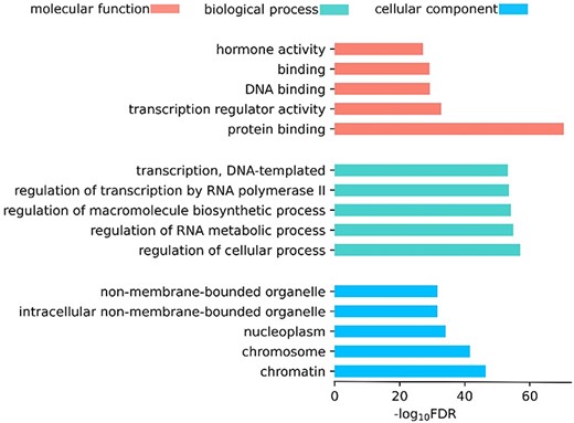
The top-5 GO items in three GO categories.
DISCUSSION
In this paper, we have developed a language-model-based method called LMDisorder to predict IDRs/IDPs in protein sequences. IDPs and IDRs are abundant in all species [65, 66], and relevant in many diseases [67, 68]. The existing profile-based methods can provide highly accurate prediction. However, they are computationally too intensive to perform genome-scale prediction due to the computational requirement for profile calculations. Here, we showed that using language model embedding as input features we can achieve speed and accuracy at the same time. For a protein with 500 residues, it takes about 15 minutes on an Nvidia GeForce RTX 3090 GPU for SPOT-Disorder2 but only one second on the same computer for LMDisorder with essentially the same performance. Meanwhile, we also tested other single-sequence-based methods, most finished within 1 to 5 seconds, because of no requirement of the time-consuming generation of sequence profiles. And compared with NetSurfP-3.0, which is the state-of-the-art language-model-based method, LMDisorder reached the equivalent or even better performance. This further proves the effectiveness of LMDisorder. In addition, the accuracy of our method remained essentially the same with the change of the protein length (Supplementary Figure S3), further indicating the robustness of our method.
One interesting observation is that the proteins with high disorder content are associated with specific biological functions. Through the enrichment analysis, we found that these proteins significantly enrich 72 GO items and many of them were supported by previous literature [6, 51, 60, 61, 69, 70]. In addition, we also discovered some new strong intrinsic-disorder-associated functions, which may be of interest for further studies.
Another observation is that combining ProtTrans and ESM did not improve over ProtTrans alone. This is a bit surprising because a recent study indicates that their combination led to an improved prediction of protein secondary structure and other tertiary structural properties [31]. This is perhaps due to the fact that disordered regions, unlike structured regions, are less conserved, and thus, evolutionary information from different language models may have captured different aspects of structural characteristics. Disorder predictions, on the other hand, are less sensitive to small intrinsic difference in the language models. In the future, we consider using the structural information predicted by AlphaFold2 [71, 72] or ESMFold [73], and then building models using graph networks [74] for further improving the performance.
In summary, this work developed a sequence-based, alignment-free method LMDisorder for protein disorder prediction. LMDisorder combines the advantages of current sequence-based and profile-based methods and greatly improves the prediction speed while ensuring high-prediction performance. The technique could be useful for highly accurate proteome-scale analysis.
LMDisorder is an alignment-free single-sequence-based protein disorder predictor that employs embedding generated by unsupervised pretrained language models as features, thus bypassing time-consuming database searches.
LMDisorder is accurate and robust, which has better performance than state-of-the-art single-sequence-based and even profile-based approaches.
The high computation efficiency of LMDisorder enables proteome-scale analysis of human, showing that proteins with high predicted disorder content were associated with specific biological functions.
LMDisorder employs transformer networks to capture the sequence patterns, especially the long-range dependencies between the residues, which is useful for protein disorder prediction.
DATA AVAILABILITY
The datasets, the source codes and the trained model are available on https://github.com/biomed-AI/LMDisorder.
FUNDING
This study has been supported by the National Key R&D Program of China [2022YFF1203100], National Natural Science Foundation of China [12126610], and by the Supercomputing facilities of Shenzhen Bay Laboratory.
Author Biographies
Yidong Song is a Ph.D. student in the School of Computer Science and Engineering at Sun Yat-sen University. His research interests include deep learning, graph neural network, protein disorder prediction and protein function prediction.
Qianmu Yuan is a Ph.D. student in the School of Computer Science and Engineering at Sun Yat-sen University. His research interests include deep learning, graph neural network and protein disorder prediction.
Sheng Chen is a Ph.D. student in the School of Computer Science and Engineering at Sun Yat-sen University. His research interests include deep learning, graph neural network and protein structure prediction.
Ken Chen is a Ph.D. student in the School of Computer Science and Engineering at Sun Yat-sen University. His research interests include deep learning, graph neural network and protein function prediction.
Yaoqi Zhou is a senior principal investigator in the Institute of Systems and Physical Biology, Shenzhen Bay Laboratory, Shenzhen, China. His research interests include protein disorder prediction, protein design and protein/RNA structure prediction.
Yuedong Yang is a professor in the School of Computer Science and Engineering at Sun Yat-sen University. Currently he focuses on integrating HPC and AI techniques for multi-scale biomedical research.
REFERENCES
Lyu H, Sha N, Qin S, et al. Manifold denoising by nonlinear robust principal component analysis, Advances in neural information processing systems 2019;
Rao R, Meier J, Sercu T, et al. Transformer protein language models are unsupervised structure learners,
Yuan Q, Chen S, Wang Y, et al. Alignment-free metal ion-binding site prediction from protein sequence through pretrained language model and multi-task learning,
Vaswani A, Shazeer N, Parmar N, et al. Attention is all you need,
Kingma DP, Ba J. Adam: A method for stochastic optimization,
Høie MH, Kiehl EN, Petersen B, et al. NetSurfP-3.0: accurate and fast prediction of protein structural features by protein language models and deep learning,
Lin Z, Akin H, Rao R, et al. Language models of protein sequences at the scale of evolution enable accurate structure prediction,
