


Abstract
Many chemicals are present in our environment, and all living species are exposed to them. However, numerous chemicals pose risks, such as developing severe diseases, if they occur at the wrong time in the wrong place. For the majority of the chemicals, these risks are not known. Chemical risk assessment and subsequent regulation of use require efficient and systematic strategies. Lab-based methods—even if high throughput—are too slow to keep up with the pace of chemical innovation. Existing computational approaches are designed for specific chemical classes or sub-problems but not usable on a large scale. Further, the application range of these approaches is limited by the low amount of available labeled training data. We present the ready-to-use and stand-alone program deepFPlearn that predicts the association between chemical structures and effects on the gene/pathway level using a combined deep learning approach. deepFPlearn uses a deep autoencoder for feature reduction before training a deep feed-forward neural network to predict the target association. We received good prediction qualities and showed that our feature compression preserves relevant chemical structural information. Using a vast chemical inventory (unlabeled data) as input for the autoencoder did not reduce our prediction quality but allowed capturing a much more comprehensive range of chemical structures. We predict meaningful—experimentally verified—associations of chemicals and effects on unseen data. deepFPlearn classifies hundreds of thousands of chemicals in seconds. We provide deepFPlearn as an open-source and flexible tool that can be easily retrained and customized to different application settings at https://github.com/yigbt/deepFPlearn.
Introduction
Exposure to a vast amount of chemicals threatens the health of humans and ecosystems. Chemical products are essential for maintaining our standard of living, and chemicals form the building blocks of life. Some chemicals are hazardous upon exposure, and their safety needs to be thoroughly evaluated. The number of chemicals that we are exposed to and the set of chemicals of anthropogenic origin has been rapidly growing from 20 million in 2002 to currently 169 million unique chemicals in The Chemical Abstracts Registry Service [8]. Many of those chemicals are not relevant for exposure since they are not used in larger quantities. The estimated number of chemicals available on the global market highly varies between 30 000 and 350 000 [6, 15, 16, 39]. The number of chemicals detected in human bodies is of similar order of magnitude. Mattingly et al. [25] compiled more than 50 000 chemicals from scientific texts in the Blood Exposome DB. Rappaport [35] defined our lifestyle and the change in environmental determinants [19, 22] rather than genetic factors as the primary cause for many chronic diseases. Contamination with anthropogenic chemicals is of similar concern in the environment [3, 7]. The NORMAN database lists |$\sim $| 3000 chemicals as emerging pollutants across Europe [28]. Chemical exposure was considered a major threat for wildlife populations [10, 17, 18]. For example, up to 26 % of aquatic species loss may be attributed to exposure to chemical mixtures [15,p . 245] and [31].
Risk assessment fails to keep up with the pace of chemical innovation. This enormous chemical exposure and observed hazards require an efficient and effective risk assessment and specific regulation of chemical use. While the EU [14] designated a ‘toxic-free environment’ a key priority, the European Environment Agency forecasts that chemical exposure will further increase [15,pp. 248–249]. For 86% of the |$\sim $|21 000 chemicals registered under REACH, the European legislation regulating industrial chemicals, the need for suitable regulatory actions still needs to be determined [12]. However, the throughput of regulatory processes is slow compared with the pace of chemical innovation. The evaluation of a chemical of concern takes 7–9 years, during which exposure may continue, under REACH regulation [15,pp. 248–249]. Also, the European Chemicals Agency [13] found that |$\sim $|70 % of the evaluated registration dossiers are incomplete or not compliant. In summary, traditional approaches to chemical regulation perform well; however, they are too slow to master the number and growth of chemicals on the market. Predictive in silico approaches may support this challenge—not necessarily by replacing experimental approaches, but by prioritizing chemicals for further evaluation.
In silico approaches predict toxicity. Different in silico approaches exist to predict toxicity. Structural alerts and rule-based models constitute a simple but powerful approach to toxicity prediction and build on using individual chemical substructures as indicators for toxicity [21]. These methods rely on either human-expertise-based or data-derived rules and are easy to interpret. However, since no mechanism enforces the completeness of rules, there is a high risk of false-negative predictions [33]. Read-across predicts the unknown toxicity by extrapolation from a set of highly related chemicals with known toxicological properties as an alternative to animal experiments. Naturally, this restricts to the subset of chemicals for which sufficient information of related chemicals is available [38]. Quantitative Structure Activity Relationships (QSAR) [33] relate molecular descriptors to toxicity or other properties of a chemical [9, 30]. QSARs are built on a set of related chemicals or expert knowledge on several chemicals’ shared mode of action or are derived from a diverse set of chemicals. Descriptors in QSARs include physicochemical properties, different molecular structure representations or properties thereof, and high-throughput screening-derived data on biological activity. A frequently used family of descriptors are molecular fingerprints that record the occurrence of local and regional substructures [24]. QSAR approaches utilize multivariate statistical models and more recently also machine learning to relate molecular descriptors to toxicity.
Machine learning in 21st-century toxicology. Toxicology experiences a paradigm shift from relying on apical endpoints in animal models to integrated strategies, combing prediction and high-throughput testing for different endpoints. Screening initiatives, e.g. the Tox21 program [37], test thousands of chemicals in hundreds of bioassays to inform on an effect on the molecular processes which are relevant in toxicity. The availability of these data enabled the development of a new variant of QSARs: the machine-learning-based prediction of the association of substances with molecular pathway responses.
The Tox21 Challenge was announced in 2014 to reveal how well independent researchers could predict the interference between chemicals and biochemical pathways given a dataset of chemical structures only. The challenge initiators provided a set of 12 000 chemicals with toxicity effect information for 12 assays along with the task to predict the effects computationally. The winning method was the DeepTox[26] pipeline with reported AUC values above 82%. In brief, they normalized the molecular representation of the chemicals, computed a large number of descriptors and trained deep learning DL models, which they evaluated on the provided test data. Later, the challenge initiators successfully validated these models on withheld data. Further, the authors observed that the models learn simple structures in the lower and more complex structures in the higher layers, as shown for image recognition. In their DL models, hidden neurons represent known molecular substructures—toxicophores, identified manually by experts for decades.
Pu et al. [32] developed eToxPred to quickly estimate the toxicity of extensive collections of low molecular weight organic chemicals. It employs a Restricted Boltzman Machine classifier and a generative probabilistic model to predict a Tox-score. The reported accuracy is 72%.
Sun et al. [36] used support vector machine and random forest single- and multilabel models to predict toxicity on the Tox21 Challenge data. They used under-sampling to resolve the problem of class imbalance in the data and reported accuracies between 74 to 81%.
Liu et al. [23] described TarPred, a web application for predicting therapeutic and side effect targets of chemicals. It is not available anymore.
The DeepChem Project [34] is a Python library that provides datasets, functions and user-contributed tutorials, intending to democratize DL for science in general and chemistry in particular. It is helpful to develop or, as a reference, to compare custom computational approaches in the field.
None of these approaches provides a ready-to-use program for classification or retraining. The main limitation of those (and other) ML approaches in toxicology is the lack of applicability to chemicals outside the training data and the availability of sufficient amounts of training data. A specific challenge is that the descriptors need to be fine-grained enough to capture the particularities of molecular substructures and coarse-grained enough to allow for ML. In particular, the representation of a chemical structure should preserve relevant information which allows for the target association, while it should also summarize structural features to reduce the degrees of freedom of the descriptor space. However, the (high) dimensionality of the features stands in considerable contrast to the (low) amount of available labeled training data.
Here, we present deepFPlearn—a ready-to-use DL program that predicts the association of chemical structures and targets on the gene/pathway level. We applied feature reduction via a deep autoencoder (AE) of a simple representation of the chemicals’ structure—the binary fingerprint of moderate size. Subsequently, we predicted the association of the encoded/compressed fingerprint representation with a deep feed-forward neural network (FNN). We overcame the domain extrapolation problem by training the autoencoder on a considerable repertoire of chemical structures and showed that the prediction quality on the subset of labeled training data remained high. Further, we demonstrated that deepFPlearn could classify selectively interacting chemicals, which have been experimentally classified recently, with significantly higher confidence than other chemicals.
Methods and data
Pearson correlation was used to evaluate the similarity of compressed features. A |$k$|-means clustering with |$k \in [2..7]$| was applied to the uncompressed features. The assigned clusters were translated to color codes in the visualizations of uncompressed and compressed features.
The deep learning tasks were implemented using the Python library of the TensorFlow framework [2,version 2.6.0] and the Scikit-learn framework [29,version 1.0.2].
We used Weights & Biases [5] for experiment tracking and hyperparameter tuning (sweep). Sweeped parameters included activation function for the hidden layers, optimizer, learning rate, learning rate decay, batch size and dropout. The supplement provides all details about the hyperparameter tuning procedure and the final selected training parameter values in section Hyperparameter tuning.
We applied a stratified train-test splitting to keep the same distribution of class labels in both, the training and the test data. For training the FNN models, we applied a stratified |$k$|-fold (default: |$k=5$|) cross-validation. We enabled early stopping and fallback mechanisms and monitored validation loss (|$val\_loss$|). The training stopped early if |$val\_loss$| did not improve by |$min_{\Delta }= 0.0001$| for a certain number of epochs (|$patience:{\mathrm{AE}} = 5$|, |$patience:{\mathrm{FNN}} = 20$|). The model’s weights were restored to the respective checkpoint model. deepFPlearn saves the model weights for each fold and the model that performed best across all |$k$| folds for subsequent prediction and further application. Training histories in terms of the values for loss, binary accuracy, area under the reciever-operator curve (AUC-ROC), precision, recall and F1 score were logged in.CSV format for each training epoch’s training and validation data. To find the optimal classification threshold we used Matthews Correlation Coefficient (MCC) as one of the unbiased evaluation metrics for imbalanced classification. MCC was calculated with an increasing threshold from 0 to 1 on the predicted values of the validation data (and their true values). Then, the threshold with maximum MCC was selected as the tuned classification threshold for each model individually. See Figure 3 C for an example.
Number and sizes of hidden layers for each trained neural network. NN—neural network; AE—autoencoder; FNN—feed-forward NN
| NN | Input | Input size | Hidden layers |
|---|---|---|---|
| AE | FP | |$L_{FP}=2048$| | 1024, 512, 256, 512, 1024 |
| FNN | FP | |$L_{FP}=2048$| | 1024, 512, 256, 128 |
| FNN | compressed FP | |$L_z=256$| | 128, 64, 32 |
| NN | Input | Input size | Hidden layers |
|---|---|---|---|
| AE | FP | |$L_{FP}=2048$| | 1024, 512, 256, 512, 1024 |
| FNN | FP | |$L_{FP}=2048$| | 1024, 512, 256, 128 |
| FNN | compressed FP | |$L_z=256$| | 128, 64, 32 |
The SELU activation function and lecun_normal weight initialization were used in hidden layers, and the Sigmoid activation function for the output layer. The model was compiled with binary cross-entropy as loss function and Adam optimizer.
Dense layers were used with the SELU activation function, lecun_normal weight initialization and AlphaDropout. The Sigmoid activation function was used for the output layer. All hidden layers were followed by a dropout layer. To reflect a potential imbalance in the training data, we introduced an initial bias of |$\log (P/N)$| (with |$P$| equal to the number of 1-values and |$N$| to the number of 0-values in the target vector) to the output layer. The FNN model was compiled using the Adam optimizer and binary cross entropy as loss function
Different datasets were collected from the literature and public databases. A manually curated dataset |$S$| was downloaded from the supplemental material of [36]. It contained chemical-target associations for 7248 chemicals and six gene targets that are involved in endocrine disruption (ED) in humans (androgen receptor (AR), estrogen receptor (ER), glucochorticoid receptor (GR), thyroid receptor (TR), PPARg and Aromatase). See supplemental Fig. S1 for an overview of these data’s size and class distributions. Initially, these data had been retrieved from bioassay data of the Tox21 program [37], and carefully transformed to binary associations by [36]: Associations were considered as not available (NA) if no bioassay data were available, and as 1 or 0, if an association between chemical and gene target had been confirmed in a bioassay or not, respectively. See [36] for details. The dataset |$S$| was extended by the artificial target ED that combines all existing target associations with a logical OR operation. Chemicals in the |$S$| dataset were identified by their SMILES string.
Further, a dataset |$D$| was generated from the 719 996 chemicals listed in the CompTox Chemistry Dashboard [40,accessed on 2020/07/13]. Chemicals in the |$D$| dataset were identified by their InChI identifiers.
For benchmarking, we downloaded two datasets from MoleculeNet [41], a database of benchmarking datasets for classification problems in molecular ML. First, we selected the Tox21 Challenge dataset—|$Tox21$|, which associates chemicals and gene targets. Second, we used the Side Effect Resource (|$SIDER$|) database that associates drugs with grouped adverse drug reactions. These datasets contained 7831 and 1427 compounds, and 12 and 27 targets, respectively, and comprised binarized associations between those compounds and the targets. We followed the recommended metric and splitting patterns [41] to generate training data from these datasets and selected targets with a 1-0-ratio of at least 0.2 and a minimal number of 200 samples in the positive class for training.
See Table 2 for an overview which of those datasets were used in which training or prediction case.
Overview of the usage of the different datasets for training or prediction
| case | train AE | use AE | train FNN | predict |
|---|---|---|---|---|
| 1 | |$S$| | - | - | - |
| 2 | |$D$| | - | - | - |
| 3 | - | - | |$S$| | - |
| 4 | - | |$S$| | |$S$| | - |
| 5 | - | |$D$| | |$S$| | - |
| 6 | - | |$D$| | |$SIDER$| | - |
| 7 | - | |$D$| | |$Tox21$| | - |
| 8 | - | |$D$| | - | |$D$| |
Implementation.deepFPlearn was implemented as a Python (version 3.9.12) package with three different usage-modes. First, convert imports the dataset (for training or prediction) and calculates molecular fingerprints for all structures from their respective SMILES or InChi representation. A data frame combines the original representation, the calculated fingerprint and all targets. It is then serialized to disc as a Pickle file to accelerate the data import for subsequent sessions. Importantly, deepFPlearn assumes that SMILES have been canonicalized and cleaned. We recommend to either use ChemAxon’s chemical structure representation toolkit (https://chemaxon.com/products/chemical-structure-representation-toolkit) or a chemical structure curation pipeline relying on RDKit [4]. The second mode is training. The neural networks can easily be (re-)trained with any dataset that associates chemical structures with an effect. All necessary information is logged during the training to validate and evaluate the trained models. The third mode is to predict the association of a provided list of chemicals with an effect using the trained models.
The user can adjust all neural network settings and the mode of action in a JSON configuration file.
Dependencies to external libraries and software are managed using a platform-independent conda (https://www.anaconda.com) environment, which we provide in the code repository. A singularity container(https://sylabs.io/) was set up that encapsulates the whole project at the state of publication for usage and reproducibility. It includes the required resources, source code, compiled package and test data.
Results
We developed the stand-alone, ready-to-use DL approach deepFPlearn to associate chemicals with gene/pathway level targets. We further evaluated the potential of feature compression to increase the applicability to substances beyond the limited amount of available training data.
Our workflow combined a pre-training strategy via a deep autoencoder to reduce the feature space and to generate a universal encoding of binary fingerpints, followed by a classification step using a deep FNN, see Figure 1.
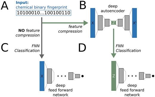
The deepFPlearn workflow. (A) The molecular fingerprints serve as input for the neural networks. (B) An AE is used to compress the fingerprints. (C) An FNN) is used for direct classification of the input. (D) An FNN is used for classification of the compressed input. Sizes of layers, activation and loss functions are different for each network and depend on the input size, see methods section.
For the FNNs, we employed 5-fold cross-validation to show that the selection of the train-test-split has no significant impact on the model performance. In particular, the standard deviation of the ROC-AUC values (calculated on the validation data) was |$\sim $|1%, see supplement Fig. S2. Therefore, we used a single stratified train-test-split to finetune and train our models.
Feature compression comprehensively reduced trainable parameters while keeping comparable classification performance. We applied different training setups: First, feature compression was disabled (no AE, Figure 1 from A to C), and FNN training used the full-length molecular fingerprints. The ratio between positive (1) and negative (0) associations differed substantially between the individual targets, see supplement Fig. S1. We introduced an initial bias to the output layer of the FNN to reflect that imbalance and selected AR, ER and the artificial target ED as subsets with an acceptable imbalance to train individual FNN models. Due to the fingerprint size of 2048, the respective hidden layer sizes of the FNN were 1024, 512, 256, 128 resulting in about 2.8e6 trainable parameters. The training stopped early before |$\sim $|100 epochs. Binary accuracy values of 0.85, 0.83, 0 .78 and ROC-AUC values of 0.81, 0.83, 0.81 were reached for AR, ER and ED, respectively. See Figure 3 A (top panels) for the training histories, and Figure 3 B (lightgray bars) for the values of precision, recall, F1 scores and further metrics that describe the performance of our FNN models. See Figure 4 A for ROC and precision-recall curves of the AR target for the classification without AE, and supplement Fig. S 3–5 for confusion matrices, ROC and precision-recall curves of all three targets.
Second, we applied feature reduction before the classification by training an AE with a latent space size of |$L_z=256$|. This reduced the respective hidden layer sizes of the FNN to 128, 64, 32, resulting in only 43.3e3 trainable parameters, which is 1.55% of the uncompressed case above. We trained both a specific AE using the (small) |$S$| dataset and a generic AE using the (large) |$D$| dataset. See Figure 1 from A over B to C. The training of the specific autoencoder stopped early at 28 epochs which is due to the small number of training samples. The validation loss reached a value of 0.026. The generic autoencoder trained for around 320 epochs and stopped at a validation loss of 0.159. See Figure 2 for the training histories and a UMAP visualization of the high-dimensional uncompressed feature space and the low-dimensional latent space of dataset |$S$|. Coloring compounds from the uncompressed and compressed space with labels calculated on the uncompressed feature space yielded similar cluster associations in the UMAP. Therefore, the AE preserves relevant (structural) information during feature compression.
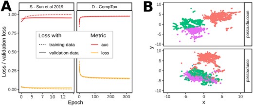
(A) ROC-AUC and loss values during training (calculated on the training and validation data after each epoch) of the specific (|$S$| – Sun et al. 2019) and the generic (|$D$| – CompTox) autoencoder. The training stopped early at 28 epochs for the specific AE—due to the small number of available training samples and reached a validation loss of 0.026. The training of the generic AE stopped at |$\sim $|320 epochs reaching a validation loss of 0.159. (B) UMAP visualizations of uncompressed and compressed representations of all compounds from |$S$| dataset; the color indicates cluster assignment of a |$k$|-means clustering with |$k=4$| on the uncompressed features.
Subsequently, we trained the FNNs and used the latent space representation as input. The training stopped early before |$\sim $|400 epochs. Binary accuracy values of 0.85, 0.80 and 0 .77 and ROC-AUC values of 0.81, 0.81 and 0.78 were reached for AR, ER and ED, respectively, when the specific AE was used to encode the fingerprints. We observed no significant discrepancy in these values when using the generic AE. In particular, we reached values of 0.85, 0.80 and 0.74 for binary accuracy, and 0.80, 0.79 and 0.76 for ROC-AUC values. Therefore, when the input features are compressed with the generic AE, the FNNs may be applied to a much more comprehensive range of molecular structures without compromising on the predictive power. See Figure 3 A (middle and lower panels) for the training histories, and Figure 3 B (medium and dark gray bars) for the values of precision, recall, F1 score and further metrics that describe the performance of our FNN models that were trained with compressed fingerprints. See Figure 4 B for ROC and precision-recall curves of the AR target for the classification with the generic AE, and supplementary Fig. 3–5 for confusion matrices, ROC and precision-recall curves for all three targets.
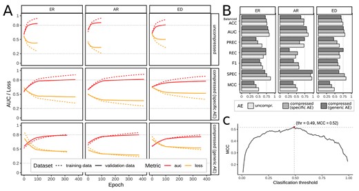
(A) Training histories of the feed forward neural networks stratified by the selected targets/models for androgen (AR) and estrogen (ER) receptors, and endocrine disruption (ED), and the degree of feature compression (uncompressed, specific AE, and generic AE); the shown metrics are ROC-AUC (red), loss (orange) calculated on the training (dotted) and validation data (solid) during training. (B) Comparison of the values of balanced accuracy (Balanced ACC), area under the receiver-operator curve (AUC), precision (PREC), recall (REC), F1 score (F1), specificity (SPEC) and MCC of the individual models using no (lightgray), the specific (medium gray) and the generic AE (dark gray). (C) MCC was calculated for increasing thresholds from 0 to 1 on the predicted validation data. The threshold with maximum MCC was selected as the individual classification threshold for each model. Example generated for model: AR, uncompressed input.
Benchmarking confirmed our strategy.
We compared the results of our strategy against the results of Sun et al. [36], the publication from which we extracted our FNN training data, the introduced approaches eToxPred [32] and DeepTox [26], and the results reported by MoleculeNet [41]. Sun et al. [36] reported balanced accuracy values in their results and we reached the same range between 74 and 81% on the same data. Pu et al. [32], Mayr et al. [26] and Wu et al. [41] reported ROC-AUC values of 72, 82 and 83%, respectively, on the Tox21 data of MoleculeNet, while our models achieved ROC-AUC values of 88%. For the SIDER dataset Wu et al. [41] reported 67% ROC-AUC values, while we reached 84%. For the MoleculeNet datasets, we also observed only a slight drop in performance when using the generic AE. In summary, our models perform either in the same range as existing approaches or better, which is satisfying compared with the increased applicability of our strategy.
deepFPlearn is ready to be applied to huge datasets. We used deepFPlearn with generic feature compression and selected the trained models for AR, ER and ED to predict associations of the |$\sim 700k$| chemicals from dataset |$D$|. For most of those compounds, the probability of acting as endocrine disruptors was not known. deepFPlearn predicted |$\sim $|60k with high prediction probability |$P>0.85$|.
From the ED predictions of dataset |$D$|, we investigated the top 200 and bottom 200 (ranked by prediction probability) and empirically investigated their biological feasibility. We found compounds among the top 200 like Estriol, 17alpha-Ethinylestradiol, 17beta-Ethinylestradiol, Mestranol, Prednisolone Dexamethasone, Betamethasone and respective derivates. These chemicals are well known to interact with the human estrogen receptors and pathways or with the glucocorticoid pathway. Interestingly, Escher et al. [11] also identified some of those to interact selectively with AR in the cell assay screenings. Also, the top 200 list contains the chemicals Ezlopitant dihydrate dihydrochloride, 5-Bromo-2, 2-diethyl-5-nitro-1,3-dioxane or Schinifoline, a metabolite of the Japanese Pepper plant Zanthoxylum schinifolium. To our knowledge, those substances have not been tested in bioassays so far. In the bottom 200 predictions (|$P<0.01$|) we found derivates of carbamic, acetic and amino acids. Those chemicals have never been discussed in the context of steroid hormone related ED as far as we know.
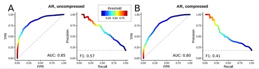
Receiver-operator (left of both panels) and precision-recall (right of both panels) curves of a single fold of the AR target without using feature compression (A), and with generic feature compression (B). The color indicates the value of the respective classification threshold. Supplemental Figure S2 depicts the standard deviations of the AUC for the five folds.
Recently, Escher et al. [11] categorized a selection of 355 out of 7968 investigated chemicals and their activity with the ED receptors AR and ER as selective (41), specific and unspecific (314, summarized as other) binders.
We predicted the associations for the subset of 339 chemicals that have not been part of our training data with and without generic feature compresssion. The models for ER and ED that were trained on the compressed fingerprints captured substantially more of the selective compounds with higher prediction probability than the models that used the uncompressed fingerprints. However, this was not true for the AR model. See Figure 5 B and C for probability distributions and counts of the ED model and supplement Fig. S6 for the comparison of all three models.
![(A) Values for all metrics calculated on the validation data for the benchmarking data sets SIDER and Tox21 summarized across all targets: balanced accuracy (Balanced ACC), area under the receiver operator curve (AUC), precision (PREC), recall (REC), F1 score (F1), specificity (SPEC) and MCC of the individual models using no (light gray), the specific (medium gray) and the generic AE (dark gray). (B)deepFPlearn prediction probabilities using the ED model with generic AE on the compounds that have been experimentally measured for quantified target association and, respectively, differentiated into selective and non-specifically acting compounds by Escher et al. [11]. Probability distributions are compared using the Kolmogorow–Smirnow test, and the significance levels for rejecting the null hypotheses that both distributions are similar was * for P-values below 0.05. (C) Comparison of the counts of predicted 1 (active) and 0 (inactive) labels for the same compounds as described in Figure B shown for the ED model.](https://oup.silverchair-cdn.com/oup/backfile/Content_public/Journal/bib/23/5/10.1093_bib_bbac257/1/m_bbac257f5.jpeg?Expires=1749223305&Signature=E5emIi0-YLcnEWJlQw0MJ9luTNACL0Lkih3wLlgTk53yZR3pCb8UPtSlwQAjMlQQt2FLRvysb5sZD1Yd9v8twiGADYci3~MKWMKsENjHCbTasKRHP8oh0ogaXA5o7T6-uIfSfZBy~u0Bvee34C4rXgqeD1n64p0A9C~XpsudqCu6SU6UgkW~w8SZcPGzasYH12hTmET73kYnaRyjYc9L9AzEEre1dnrc1wSHE3kfc5gSZHAYlp8JXKueQ9J0NgnXMpvcipJonfziNs9tmuvtThrroozZps4cf1dnH9B8CwOZwjEA54E0N8Vead2SRiQh4O5ZgG2CiDYqVOb7oE~H5Q__&Key-Pair-Id=APKAIE5G5CRDK6RD3PGA)
(A) Values for all metrics calculated on the validation data for the benchmarking data sets SIDER and Tox21 summarized across all targets: balanced accuracy (Balanced ACC), area under the receiver operator curve (AUC), precision (PREC), recall (REC), F1 score (F1), specificity (SPEC) and MCC of the individual models using no (light gray), the specific (medium gray) and the generic AE (dark gray). (B)deepFPlearn prediction probabilities using the ED model with generic AE on the compounds that have been experimentally measured for quantified target association and, respectively, differentiated into selective and non-specifically acting compounds by Escher et al. [11]. Probability distributions are compared using the Kolmogorow–Smirnow test, and the significance levels for rejecting the null hypotheses that both distributions are similar was * for P-values below 0.05. (C) Comparison of the counts of predicted 1 (active) and 0 (inactive) labels for the same compounds as described in Figure B shown for the ED model.
Discussion
There is a great need for systematic prediction of chemical-effect associations in toxicology. They are required to prioritize chemicals for experimental screening, a smart selection of chemicals for monitoring and the design of novel chemicals. Several approaches and implementations exist that partially address these challenges. However, no tools for large-scale application are available, and the option for retraining with additional data sets is absent. While MoleculeNet [41] and Deepchem [34] provide capable frameworks for developing learning applications on chemicals, readily applicable tools, e.g. for predicting ED, are missing.
With deepFPlearn we present an application to investigate sets of chemicals for their potential associations to gene targets involved in ED. It is a DL approach with the possibility of training custom models to predict different associations of interest.
The small number of labeled training data is in contrast to the high number of features necessary to describe a chemical’s molecular structure. Also, the natural interaction of chemicals and biomolecules is biased toward ‘no interaction’ (label of 0) such that the data suffer from a substantial imbalance between 1 and 0 labels. Assessing the association of chemicals and biomolecules requires measuring a range of concentrations per substance and assay and thus poses a substantial effort even with high-throughput technologies. Since the number of substances with measured associations is small compared with the universe of chemicals, there is a lack of labeled training data. Due to the high speed at which new chemicals are developed, this situation will not change in the foreseeable future. To make things worse, many positive associations (label of 1) are potentially wrong due to mistakes during screening result interpretation. Examples are unclear effect thresholds, high variability in the experimental designs and limitations in the statistics of modeling the observed effect. The imbalance of the training data together with a large number of parameters can easily lead to overfitting. This is reflected by a large discrepancy between the training and validation loss, which we still observe in the cases where we do not use feature compression. However, our strategy to initialize the output layer of the FNN with the correct bias to reflect the imbalanced class distribution, which has been recently proposed by [1], our extended hyperparameter tuning and the application of fallback mechanisms, reduced overfitting also for the uncompressed FNN. In supplemental Figure S8 we show how the model can be driven into overfitting when one of these strategies is disabled.
We reduced the discrepancy between large descriptor size and the limited training data by compressing features with a deep autoencoder. Further, this reduced the large number of trainable parameters to 1.55|$\%$| of the networks that do not use an AE. Using a large repertoire of chemicals for training the AE further improved the domain extrapolation without reducing the predictive power of the subsequent classification. We tested different training situations, (i) without feature compression, (ii) feature compression with a subset of chemicals (specific AE) and (iii) feature compression with a large set of chemicals (generic AE). We reached good training performances with ROC-AUC values above 80%, with satisfying sensitivity up to 75%, and specificity up to 97%.
Using the benchmark datasets from MoleculeNet, and reported binary accuracies and ROC-AUC values from other approaches that used the same data sets we showed that deepFPlearn performed comparably or better. However, those methods also demand significant adjustments to the training data to cope with imbalance. We found that our predictions with the generic AE captured more of the compounds that have been experimentally analyzed and classified by [11] than the models trained on the uncompressed fingerprints, which verifies our assumption on predicting unseen data.
deepFPlearn allows for selecting different usage modes depending on the classification problem: If the compounds to be classified are expected to reside within the domain of the training data the FNN without AE provides superior classification performance. However, given the overall comparable accuracy of deepFPlearn when pre-training on a large data set, we consider this the more robust, computationally efficient and generally more applicable approach in particular for large, heterogeneous and imbalanced data.
The quality of our predictions is also high on the large CompTox dataset. Among the top 1–associated predictions were chemicals that are well known to interact with human estrogen or the glucocorticoid receptor or related pathways. Likewise, among the respective top 0–associated predictions were chemicals that have never been discussed to be involved in ED, which further enhances the confidence in our models.
Our high values for specificity also suggest an application of deepFPlearn to predict secondary effects in drug design.
The deepFPlearn results on the chemicals experimentally classified as selective and unspecific also confirmed our prediction quality. Although a relatively broad distribution of prediction probabilities for selective binders suggests that there is still room for methodological improvement, many of the chemicals predicted with a very high probability are indeed selective binders.
We suggest a more detailed investigation of the predicted associations and experimental validation in upcoming studies to confirm or decline effects in endocrine disruption.
Conclusion
With deepFPlearn we model the associations between chemical structures and effects on the gene/pathway level with a deep learning approach.
In contrast to existing approaches and implementations, deepFPlearn is a ready-to-use tool. It comes as a stand-alone Python software package and (additionally) wrapped in a Singularity Container to overcome the dependency on the operating system and required software. deepFPlearn can capture a much more comprehensive range of substances than those contained in the training data of the classification network. It can be applied to classify hundreds of thousands of chemicals in seconds. Moreover, with its different application modes, we provide the flexibility to train custom models with any meaningful dataset that associates chemicals with an effect. deepFPlearn substantially contributes to the systematic in silico investigation of chemicals, even for data-driven hypothesis generation on novel substance-effect associations. With deepFPlearn we can cope with the large, constantly and rapidly growing chemical universe and support prioritization of chemicals for experimental testing, assist in the smart selection of chemicals for monitoring and contribute to the sustainable design of the future chemicals.
All living species are exposed to a vast amount (and mixtures) of chemicals; many pose risks; this risk is not known for the majority.
To support the lab-based risk assessment and subsequent regulation of use, prioritize chemicals for experimental design and hypothesis generation, efficient and systematic tools that can evaluate the chemical-effect association on a large scale are required, but are not available so far.
We present the ready-to-use deep learning application deepFPlearn that predicts the association between the chemical’s molecular structure and the observed effect on the gene/pathway level.
We solved the discrepancy between large feature space describing the molecular structure and the low amount of labeled training data with a pre-training strategy for feature compression on the chemical inventory.
We confirmed the good performance and high prediction quality of deepFPlearn with benchmarking and experimentally validated datasets.
Availability of source code and data
The source code is available in a git repository at github: https://github.com/yigbt/deepFPlearn under the terms of the UFZ license, which is based on GNU General Public License as published by the Free Software Foundation version 3 or later. We refer to this repository for installation and usage instructions. For ease of use we also provide Docker and Singularity containers, which is accessible via this repository. These containers also contain the data used for training the models.
Author contributions statement
J.S. and J.H. planned the study; J.S. and C.L. defined the neural network architectures; J.S. preprocessed all data; J.S. and P.S. implemented the software package and analyzed the results; M.B. and P.S. built the singularity container and all github actions; all authors wrote the manuscript. All authors read and approved the final manuscript.
Acknowledgments
The authors are grateful to Martin Krauss for helpful discussions.
Funding
This work was supported in part by the Helmholtz. AI project XAI-graph and by the CEFIC Long Range Initiative through funding the project C5 - XomeTox, the Helmholtz program ``Changing Earth - Sustaining our Future'' topic 9, and the Horizon Europe Partnership for the Assessment of Risk from Chemicals.
Author Biographies
Jana Schor heads the Group Data Science in Bioinformatics, Department of Computational Biology at the Helmholtz-Centre for Environmental Research GmbH – UFZ. She has a strong background in computer science and bioinformatics. Jana implements state-of-the-art data science methods, and promotes the principles of reproducible research in the field of computational toxicology.
Jörg Hackermüller heads the Department of Computational Biology at the Helmholtz-Centre for Environmental Research GmbH – UFZ and is professor of Computational Biology at Leipzig University. His research group develops bioinformatics, systems biology, and data science approaches to advance mechanistic understanding in toxicology and environmental health. Jörg has a background in computational biology and biochemistry.
