


Abstract
There is growing evidence showing that the dysregulations of miRNAs cause diseases through various kinds of the underlying mechanism. Thus, predicting the multiple-category associations between microRNAs (miRNAs) and diseases plays an important role in investigating the roles of miRNAs in diseases. Moreover, in contrast with traditional biological experiments which are time-consuming and expensive, computational approaches for the prediction of multicategory miRNA–disease associations are time-saving and cost-effective that are highly desired for us.
We present a novel data-driven end-to-end learning-based method of neural multiple-category miRNA–disease association prediction (NMCMDA) for predicting multiple-category miRNA–disease associations. The NMCMDA has two main components: (i) encoder operates directly on the miRNA–disease heterogeneous network and leverages Graph Neural Network to learn miRNA and disease latent representations, respectively. (ii) Decoder yields miRNA–disease association scores with the learned latent representations as input. Various kinds of encoders and decoders are proposed for NMCMDA. Finally, the NMCMDA with the encoder of Relational Graph Convolutional Network and the neural multirelational decoder (NMR-RGCN) achieves the best prediction performance. We compared the NMCMDA with other baselines on three experimental datasets. The experimental results show that the NMR-RGCN is significantly superior to the state-of-the-art method TDRC in terms of Top-1 precision, Top-1 Recall, and Top-1 F1. Additionally, case studies are provided for two high-risk human diseases (namely, breast cancer and lung cancer) and we also provide the prediction and validation of top-10 miRNA–disease-category associations based on all known data of HMDD v3.2, which further validate the effectiveness and feasibility of the proposed method.
Introduction
MiRNAs are a sort of small endogenous noncoding RNAs (21–24 nucleotides in length), which play vital roles in multiple biological processes [1–3]. The dysfunction of miRNAs and their target mRNAs may result in various human diseases [4]. For instance, the expression level of let-7 in lung cancer was markedly reduced, confirming that miRNAs are closely related to the occurrence of tumors [5]; abnormal expression of mir-107 may affect the activity of BACE1 (β-secretase 1) to cause Alzheimer disease [6]. Therefore, the identification of disease-related miRNAs can contribute to the pathological study of diseases and disease biomarker detection [7–11]. As the identification of the associations between miRNAs and diseases using biological experiments is time-consuming and expensive [12], in the last few years many computational methods [13–25] have been developed to determine the potential associations between miRNAs and diseases (hereafter abbreviate MDA).
Most of the existing research works, such as [13–25], mainly focused on the binary association prediction (i.e. only predicting the existence of miRNA–disease association) and indeed achieved good results. However, more and more evidence shows that the dysregulations of miRNAs cause diseases through various kinds of underlying mechanisms [26–29]. For example, epigenetic alterations may lead to abnormal expression of miRNAs to cause diseases: the promoter methylation reduces the expression levels of mir-17 ~ 92 cluster, which results in bronchopulmonary dysplasia [30]; the interactions between miRNAs and their targets are related to many diseases: mir-101 inhibits the interaction between fibroblasts and cancer cells through targeting CXCL12 which affects the proliferation of lung cancer cells [31]. Furthermore, the same miRNA may associate with the same disease through different association mechanism. For instance, mir-101 affects lung cancer via targeting CXCL12 as aforementioned, meanwhile, mir-101 also suppresses lung cancer by inhibiting DNA methylation in lung cancer cells [32]. The specific category of miRNA–disease association cannot be identified with the aforementioned methods. Thus, identifying multiple categories of miRNA–disease associations can not only provide more detailed potential associations between miRNAs and diseases but also further deeper our understanding of the molecular basis of diseases in the level of miRNAs.
In the past years, only a few research works have been devoted to identifying multiple categories of miRNA–disease associations (MCMDA). Chen et al. [33] first study the problem of MCMDA. In their study, the model of Restricted Boltzmann machine for multiple types of miRNA–disease association prediction (RBMMMDA) was developed to predict four different types of miRNA–disease associations. Based on this model, not only new miRNA–disease associations but also corresponding association types could be obtained. Zhang et al. [34] proposed a semisupervised model called the network-based label propagation algorithm (NLPMMDA) is proposed to infer multiple types of miRNA–disease associations by mutual information derived from the heterogeneous network. Note that the aforementioned two research works developed their methods based on the Human MicroRNA Disease Database 2.0 [26] (hereafter abbreviate HMDD v2.0) released in 2013.
The recently released Human MicroRNA Disease Database 3.0 [27] (the latest version is HMDD v3.2) provided six generalized categories of associations, including the miRNA–disease associations from the evidence of genetics, epigenetics, circulation miRNAs, tissue, miRNA-target and other interactions, respectively. These associations cover 20 different categories of detailed association evidence codes. HMDD v3.2 significantly extends HMDD v2.0 in miRNA, disease items, miRNA–disease association entries and provides more association categories information. This provides an opportunity for developing new data-driven MCMDA methods.
Recently, oriented to the HMDD v3.2 dataset, Huang et al. [35] represented the multicategory miRNA–disease associations as a tensor and formulate the multicategory miRNA–disease association prediction as a tensor completion task. They proposed a novel tensor decomposition-based model, named tensor decomposition with relational constraints (TDRC) to solve MCMDA, which incorporates the information of miRNA–miRNA similarity and disease–disease similarity as decomposition constraints. Experimental results show TDRC significantly outperformed the other baselines [33–35].
Despite the effectiveness of TDRC and other methods for MCMDA, there are still some limitations to current research results. First, miRNA–disease association prediction relies on the hypothesis that functionally similar miRNAs are often associated with phenotypically similar diseases and vice versa. Therefore, the similarity of information both for miRNAs and diseases is crucial for accurate prediction. However, the RBMMMDA [33] merely made use of known multiple categories of miRNA–disease associations and did not consider the similarity of information between miRNAs (diseases). This restricts the prediction performance of RBMMMDA. Also, although TDRC [35] takes the information of miRNA–miRNA similarity and disease–disease similarity as decomposition constraints, the technical framework of tensor decomposition cannot easily use miRNA and disease feature information from other sources.
Second, the NLPMMDA [34] treats predicting one category of miRNA–disease association as an independent task and therefore ignores the correlations between association categories. However, different association categories may be highly associated with each other. TDRC [35] uses tensor decomposition to capture the complicated multilinear relationship between miRNAs, diseases and association categories through the tensor multiplications to overcome the aforementioned limitations. However, TDRC is essentially a multilinear method and may not be enough to capture the complex and nonlinear interactions between the features of miRNAs and diseases.
To overcome the aforementioned limitations of current approaches for MCMDA, we present a novel data-driven end-to-end learning-based method of neural multiple-category miRNA–disease association prediction (NMCMDA) to address the problem of MCMDA. The NMCMDA has two main components: Encoder operates directly on the miRNA–disease heterogeneous network and leverages Graph Neural Network to learn miRNA and disease latent representations, respectively. Decoder yields miRNA–disease association scores with the learned latent representations as input. Various kinds of encoders and decoders are proposed in this study. Finally, NMCMDA with the encoder of multiple-relational Graph Convolutional Network and the neural multiple-relational decoder (NMR-RGCN) achieves the best prediction performance. We compared the proposed method with other baselines on three experimental datasets. The experimental results show that the NMR-RGCN is significantly superior to the state-of-the-art method TDRC in terms of Top-1 precision, Top-1 Recall and Top-1 F1. Additionally, case studies are provided for two high-risk human diseases (breast cancer and lung cancer) and we also provide the prediction and validation of top-10 miRNA–disease-category associations based on all known data of HMDD v3.2, which further validate the effectiveness and feasibility of the proposed method.
Materials
The Human MiRNA Disease Database (HMDD) [26, 27] is a database that contains experimentally verified human miRNA–disease associations. Since the first version was released in 2007, HMDD has served as an important data source for the research of miRNA–disease associations. HMDD provides multiple types of evidence for associations between miRNAs and diseases which play important roles in understanding the mechanisms underlying the dysregulations of miRNAs causing diseases. These association data provide an important data basis for the research of data-driven MDA. Besides, other side information, such as miRNA–miRNA similarity and disease–disease similarity, can be used to improve MDA prediction performance.
In what follows, we first introduce the details about multiple categories of associations in HMDD. Then, we discuss the methods of constructing the miRNA–miRNA similarity and disease–disease similarity from the corresponding data sources.
Multiple categories of MiRNA–disease associations
The recently released HMDD v3.2 provides six generalized categories of associations (Genetics, Epigenetics, Target, Circulation, Tissue and Other) covering 20 types of detailed evidence codes. After preprocessing and removing duplications, we finally obtain the following datasets:
MCD-6 is from HMDD v3.2, which contains above mentioned 6 categories, including 25 849 associations between 894 diseases and 1208 miRNAs.
MCD-20 is also obtained from HMDD v3.2 which contains 20 detailed evidence codes for associations between 894 diseases and 1208 miRNAs.
In addition, the following datasets are adopted as experimental datasets to compare the performance with our proposed methods.
MCD-4 is obtained from HMDD v2.0 [26] released in 2013. MCD-4 contains four categories (Genetics, Epigenetics, Circulation, and Target) of associations between 324 miRNAs and 169 diseases.
TDRC v2.0 and TDRC v3.2 are released and provided by the published paper [35]. TDRC v2.0 contains four-category (Genetics, Epigenetics, Circulation and Target) associations between 169 diseases and 324 miRNAs. TDRC v3.2 contains five-category (Genetics, Epigenetics, Circulation, Target, and Tissue) associations between 447 diseases and 713 miRNAs.
The statistics of these datasets are shown in Table 1.
Statistics of the datasets used in this study
| Data | #d | #m | #c | #m–d | Sr |
|---|---|---|---|---|---|
| MCD-6 | 894 | 1208 | 6 | 25849 | 0.399% |
| MCD-20 | 894 | 1208 | 20 | 25849 | 0.120% |
| MCD-4 | 171 | 385 | 4 | 2003 | 0.761% |
| TDRC v2.0 | 169 | 324 | 4 | 1675 | 0.681% |
| TDRC v3.2 | 447 | 713 | 5 | 16341 | 1.025% |
| Data | #d | #m | #c | #m–d | Sr |
|---|---|---|---|---|---|
| MCD-6 | 894 | 1208 | 6 | 25849 | 0.399% |
| MCD-20 | 894 | 1208 | 20 | 25849 | 0.120% |
| MCD-4 | 171 | 385 | 4 | 2003 | 0.761% |
| TDRC v2.0 | 169 | 324 | 4 | 1675 | 0.681% |
| TDRC v3.2 | 447 | 713 | 5 | 16341 | 1.025% |
#d, disease number; #m, miRNA number; #c, category number; #m–d, association number; Sr, sparsity rate.
We observe that all miRNA–disease associations in HMDD can be divided into different categories. Supplementary Table 1 gives the statistics of m–d associations of different categories in MCD-6, MCD-4 and TDRC v3.2, respectively. On the other hand, some miRNA–disease associations may occur simultaneously in different categories. Supplementary Table 2 gives the statistics of disease–miRNA associations appearing simultaneously in different categories. We can see that although many miRNA–disease associations belong to only one category, some still belong to two or more categories. This further increases the challenge of accurate predictions.
MiRNA–miRNA similarity
With |$\mathrm{MS}(i,j)$|, the miRNA functional similarity matrix is denoted by |${\mathbf{A}}_{\mathrm{m}}\in{\mathbb{R}}^{m\times m}$|and constructed by |${[{\mathbf{A}}_{\mathrm{m}}]}_{ij}=\mathrm{MS}(i,j)$|.
Disease–disease similarity
Intuitively, |${\mathrm{dS}}_1(i,j)$| is higher if the larger part of DAG is shared by i and j.
As disease similarity measures calculated using |${\mathrm{dS}}_1$| and |${\mathrm{dS}}_2$| are both from the MeSH database, it provides only a part of the entries in diseases semantic similarity matrix. Hence, the Gaussian interaction profile kernel similarity was adopted to complement the remaining disease similarity entries.
Methods
In this section, we first formulate the multicategory miRNA–disease association prediction as a tensor completion problem. Then, an end-to-end learning-based prediction model is proposed to solve the problem.
Problem formulation
Multicategory associations could be organized into a binary three-way tensor|$\mathbf{\mathcal{T}}\in{\{0,1\}}^{|M|\times |D|\times |C|}$|, where|$|M|=m$|,|$|D|=n$| and |$|C|=R$| represent the size of the set of miRNAs, diseases and association categories, respectively. The |$r\in \{1,2,\dots, R\}$| slice of |$\mathbf{\mathcal{T}}$| is an adjacent matrix |${\mathbf{T}}^{(r)}\in{\{0,1\}}^{|M|\times |D|}$| with 0–1 entries with regard to the |$r$|-category known miRNA–disease associations, where|${\mathbf{T}}^{(r)}(i,j)=1$| if a miRNA |$i\in M$| is associated with a disease |$j\in D$| in the |$r$|-evidence category. |${\mathbf{T}}^{(r)}(i,j)=0$| if the association between a miRNA |$i$| and a disease |$j$| is unknown or unobserved.
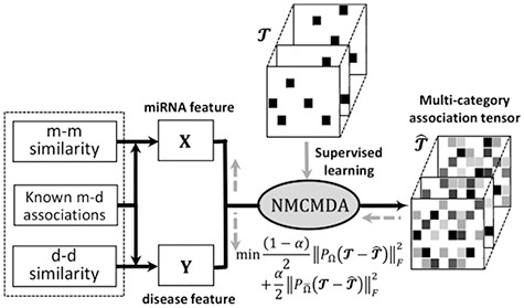
The general flowchart of MCMDA, which is mainly composed of two steps: (Step1) The feature representation learning modular learns miRNA and disease latent representations with similarity information and the known associations as input. (Step2) Prediction modular yields multicategory association scores. Totally, MCMDA is formulated as a tensor completion problem with side information.
When we solve the MCMDA defined by Equation (12), some questions must be answered. First, what are the appropriate feature representations for miRNAs and diseases? How can the feature matrices |$\mathbf{X}$| and |$\mathbf{Y}$| be obtained by exploiting the miRNA–miRNA similarity, disease–disease similarity, and the known different categories of miRNA–disease associations? Second, how to capture the dependency relationship between the latent feature representation and different association categories and establish the well-designed parameterized model to yield prediction score tensor|$\hat{\mathbf{\mathcal{T}}}$|? Finally, can we integrate the above two modules effectively to build an end-to-end learning pipeline from miRNA and disease feature representations learning to multiple-association prediction?
To answer these questions and solve the problem of MCMDA, in this paper, we develop an end-to-end learning-based prediction model that operates directly on a miRNA–disease multirelational heterogeneous graph. Generally, our proposed model has two main components: (i) encoder leverages graph neural network on the miRNA–disease multirelational heterogeneous graph to learn miRNA and disease latent representations, respectively. (ii) Decoder yields miRNA–disease association scores with the learned latent representations as input. In the following, we discuss the details of two components.
Encoders for latent feature of MiRNA and disease
In this subsection, two kinds of encoders are proposed to obtain latent features of miRNAs and diseases. The first is GCN-encoder which maps the nodes of miRNAs and diseases to the latent features by using graph convolutional network on the miRNA–miRNA similarity network and disease–disease similarity network, respectively. The second is RGCN-encoder which yields latent features by both exploiting similarity networks and the known different categories of miRNA–disease associations.
GCN-encoder
Let us start with discussing the details of the GCN-encoder. The basic assumption for miRNA–disease association prediction is that functionally similar miRNAs are more likely to be associated with phenotypically similar diseases, and vice versa. Therefore, similarity information among miRNAs and diseases are crucial for MDA. Here, the miRNA and disease latent feature representations are yielded by leveraging Graph Convolutional Network (GCN) [39] on the miRNA (or disease) similarity networks.
Let |${G}_m$| and |${G}_d$| be the miRNA functional similarity network and disease semantic similarity network, respectively. |${\mathbf{A}}_{\mathrm{m}}$| denotes the adjacent matrix for |${G}_m$| and |${\mathbf{A}}_d$| for |${G}_d$|. |$|{V}_m|=m$| and |$|{V}_d|=n$| denote the size of the node set |${V}_m$| over |${G}_m$| and |${V}_d$| over |${G}_d,$| respectively. Let |$\mathbf{X}$| and |$\mathbf{Y}$| be the initial features on the set of nodes of the graph |${G}_m$| and |${G}_d$|, respectively. GCN learns a node |$i$|’s feature by exploiting hierarchically aggregating feature information from |$i$|’s neighborhood. Next, we introduced the method of learning features for miRNAs over |${G}_m$|. The way of learning features for diseases over |${G}_d$| is a similar process.
Thus, considering a miRNA functional similarity network and a disease semantic similarity network, starting from the randomly initialized embedding |$\mathbf{X}$| and |$\mathbf{Y}$|, GCN transforms the features in a layer-by-layer manner and finally outputs |${\mathbf{X}}^{(L)}$| and |${\mathbf{Y}}^{(L)}$|. These learned features will be used as the input for the downstream multicategory association prediction model.
Note that GCN-encoder neglects the known multiple categories of associations between miRNA and disease when yielding the latent feature. Naturally, the quality of latent features may be further improved by considering these associations. In fact, miRNA, disease similarity networks, and the known miRNA–disease associations together form heterogeneous multiple relational networks. Hence, we can exploit the Relational Graph Convolutional Network [40] to yield the latent feature representations.
RGCN-encoder
Similar to GCN-encoder, we can stack multilayer RGCN feature aggregation operations to form an RGCN encoder. The RGCN-encoders for miRNA and disease are denoted by |$\mathrm{R}{\mathrm{GCN}}_m^{(L)}(\mathbf{X};{\boldsymbol{\Theta}}_m)$| and |$\mathrm{R}{\mathrm{GCN}}_d^{(L)}(\mathbf{Y};{\boldsymbol{\Theta}}_d)$|, respectively.
Different from the idea of GCN-encoder, the RGCN-encoder fully considers the different types of relations between miRNAs and diseases, such as miRNA–miRNA similarities, disease–disease similarities and multiple categories of miRNA–disease associations, and transforms the features into different types of feature space with relation-specific filter parameters matrix and finally aggregate different type features. We will demonstrate that this will improve the quality of representation learning via experimental results.
Decoders score multicategory miRNA–disease association
In our proposed prediction model, an association prediction score for the |$r$|-category is obtained by a decoder which is a parameterized score function |${\mathrm{Dec}}^{(r)}(\mathbf{X},\mathbf{Y};\mathbf{\mathcal{W}}):{\mathbb{R}}^m\times R\times{\mathbb{R}}^d\to \mathbb{R}$| where |$\mathbf{X},\mathbf{Y}$| are the encoded miRNA and disease features, respectively. In this paper, we introduce the following three different decoders.
We observe that the diagonal matrix |${\mathbf{D}}^{(r)}$| in the DistMult decoder only captures the interactions between miRNAs and diseases under the specific |$r$| category. However, as shown in Supplementary Table 2 there may be associations across different categories. To this end, we extend |${\mathrm{Dec}}_{\mathrm{DistMult}}^{(r)}$| by incorporating a trainable parameter matrix|$\mathbf{G}$| into it and propose the following Linear Multi-Relational decoder.
Both |${\mathrm{Dec}}_{\mathrm{DistMult}}^{(r)}$| and |${\mathrm{Dec}}_{\mathrm{LMR}}^{(r)}$| are bilinear decoders. Inspired by the idea of NIMCGCN [25], we proposed a novel method of neural multicategory association score model to capture the deeper and nonlinear interactions between the latent features of miRNAs and diseases.
NMR-decoder (denoted by |${\mathrm{Dec}}_{\mathrm{NMR}}^{(r)}$|) represents a Neural Multi-Relational decoder. In the following, we will take miRNA as an example to show the idea of |${\mathrm{Dec}}_{\mathrm{NMR}}^{(r)}$|. The same idea can be applied to diseases.
A nonlinear transformation from |$k$|-layer to |$(k+1)$|-layer in |${\varphi}_m^{(r;K)}$|is defined as |${\mathbf{X}}^{(r;k+1)}=\sigma \left({\mathbf{W}}_m^{(r;k)}{\mathbf{X}}^{(r;k)}+{\mathbf{b}}_m^{(r;k)}\right)$| where |${\mathbf{X}}^{(r;k)}$| is the feature matrix at k-layer, |${\mathbf{W}}_m^{(r;k)}$| is the transformation parameter matrix and |${\mathbf{b}}_m^{(r;k)}$| is the bias vector. |$\sigma (\cdot )$| is a nonlinear active function. We denote all trainable parameters by |${\boldsymbol{\Psi}}_m=\{{\boldsymbol{\Psi}}_m^{(1)},\dots{\boldsymbol{\Psi}}_m^{(r)},\dots, {\boldsymbol{\Psi}}_m^{(R)}\}$| where |${\boldsymbol{\Psi}}_m^{(r)}=\{{\mathbf{W}}_m^{(r;0)},\dots, {\mathbf{W}}_m^{(r;K)},{\mathbf{b}}_m^{(r;0)},\dots, {\mathbf{b}}_m^{(r;K)}\}$| is the parameters involved in |${\varphi}_m^{(r;K)}$|.
End-to-end learning models
The various encoders and decoders described in the previous subsection can be combined into specific MCMDA prediction models. For example, when using RGCN as encoder and NMR as decoder, we get NMR-RGCN. Similarly, we also have NMR-GCN, LMR-RGCN and so on. Next, we introduce a general loss function which can be used as the loss function of different encoder–decoder combinations.
It is worth mentioning that an encoder and a decoder are integrated into a unified end-to-end neural network learning framework. Specifically, GNN encoder is first leveraged to learn miRNA and disease features over a miRNA–disease heterogeneous information network, respectively. Then, decoder receives the learned latent features to take further transformations. The final prediction scores are obtained through the dot product of the transformed features. All parameters |$\mathbf{\mathcal{W}}$| involved in encoders and decoders are simultaneously optimized via a gradient descent with adaptive moment estimation [42]. Figure 2 demonstrates the flowchart of NMR-RGCN.
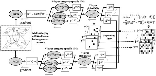
The flowchart of the NMR-RGCN, which is a specific model of Neural Multi-Category MiRNA-Disease Association prediction, i.e. NMCMDA with Neural Multi-Relational decoder and Relational Graph Convolutional Network encoder. NMR-RGCN operates directly on the miRNA–disease heterogeneous network and leverages RGCN to learn miRNA and disease latent representations, respectively. Then, neural multirelational decoder yields miRNA–disease association scores with the learned latent representations as input. The representation learning encoder and the prediction score decoder are integrated into a unified end-to-end neural network learning framework.
Results and discussion
Experimental setup
The experimental code is implemented based on the open-source machine learning framework Pytorch (https://pytorch.org). Graph neural network encoders are implemented based on the open-source deep learning on graph library (https://www.dgl.ai/). All experiments are carried on Windows 10 operation system with a Dell Precision T5820 workstation computer of an intel W-2145 8 cores, 3.7GHz CPU and 64G memory.
In this study, two following evaluation settings are setup.
(1) |${\mathbf{CV}}_{\mathbf{triplet}}{:}$| We randomly split all experimentally verified miRNA–disease-category triplets (as positive samples) into 10 subsets. In each fold, one subset and an equal-sized set of randomly sampled unknown triplets (as negative samples) as a testing set, the remaining subsets and an equal-sized set of randomly sampled unknown samples were used as a training set. Note that we were extremely careful to ensure the train and test sets did not include each other. The area under the precision-recall (AUPR) curve and the area under the receiver operating characteristic (AUC) curve were used to evaluate the prediction performance of all prediction methods.
(2) |${\mathbf{CV}}_{\mathbf{category}}{:}$| Every miRNA–disease pair is connected through zero, one or more relation types in our modeling problem. In this case, we randomly split all miRNA–disease pairs which are connected with not less than one type of association into ten subsets. In each fold, one subset as the testing set in turn, and the rest subsets as a training set. Each miRNA–disease pair in the test set is ranked under all association categories according to the predicted score. Then we consider the category with the highest score as the model prediction result for the test sample and calculate the precision (Top-1), recall (Top-1), f1-score (Top-1).
Comparing with the binary miRNA–disease association prediction, we pay more attention to the prediction of the associated category in the problem of miRNA–disease multirelational prediction which is exactly the test goal of |${\mathbf{CV}}_{\mathbf{category}}$|, so we regard |${\mathbf{CV}}_{\mathbf{category}}$| as the primary experimental setting.
Performance analysis of various encoder–decoder combinations
Our proposed model is totally based on two components, i.e. encoders and decoders. Various encoders are presented to obtain the feature representations of input data. With the input of encoded features, several decoders are presented to produce multiple categories of association scores.
In this subsection, we conduct extensive experiments on MCD-6 and MCD-20 datasets to systematically compare the performances of NMR-RGCN (NMR as a decoder and RGCN as an encoder, the meanings of other notations are similar), DistMult-RGCN, LMR-RGCN, NMR-GCN. The compared results are shown in Tables 2 and 3.
Experiment results of the various encoder–decoder combinations on MCD-6 dataset
| MCD-6 dataset | CVtriplet | CVcategory | |||
|---|---|---|---|---|---|
| AUPR | AUC | Top-1 P | Top-1 R | Top-1 F1 | |
| NMR-GCN | 0.9467 | 0.9494 | 0.5116 | 0.3690 | 0.4288 |
| DistMult-RGCN | 0.9423 | 0.9371 | 0.4059 | 0.2912 | 0.3391 |
| LMR-RGCN | 0.9525 | 0.9501 | 0.5232 | 0.3722 | 0.4350 |
| NMR-RGCN | 0.9533 | 0.9521 | 0.5522 | 0.3967 | 0.4617 |
Experiment results of the various encoder–decoder combinations on MCD-20 dataset
| MCD-20 dataset | CVtriplet | CVcategory | |||
|---|---|---|---|---|---|
| AUPR | AUC | Top-1 P | Top-1 R | Top-1 F1 | |
| NMR-GCN | 0.9419 | 0.9370 | 0.3593 | 0.2565 | 0.2933 |
| DistMult-RGCN | 0.9425 | 0.9374 | 0.1961 | 0.0516 | 0.0817 |
| LMR-RGCN | 0.9479 | 0.9505 | 0.3666 | 0.2729 | 0.3129 |
| NMR-RGCN | 0.9480 | 0.9527 | 0.4230 | 0.2893 | 0.3436 |
The effect of the biased item |$\boldsymbol{\alpha}$| in the loss function on the performance of NMR-RGCN.
The effect of the layer number of RGCN encoders |$\mathbf{L}$| on the performance of NMR-RGCN.
The effect of the number of neural multicategory layer on the performance of NMR-RGCN
| Top-1 P | Top-1 R | Top-1 F1 | |
| (|$K=1,\mathrm{LMR}$|) + (|$H=1,\mathrm{LMR}$|) | 0.3854 | 0.3015 | 0.3383 |
| (|$K=1,\mathrm{NMR}$|) + (|$H=1,\mathrm{NMR}$|) | 0.5173 | 0.3841 | 0.4409 |
| (|$K=1,\mathrm{NMR}$|) | 0.3501 | 0.2748 | 0.3079 |
| (|$K=2,\mathrm{NMR}$|) + (|$H=1,\mathrm{NMR}$|) | 0.5452 | 0.3998 | 0.4613 |
| (|$K=3,\mathrm{NMR}$|) + (|$H=1,\mathrm{NMR}$|) | 0.5531 | 0.4059 | 0.4682 |
| (|$K=4,\mathrm{NMR}$|) + (|$H=1,\mathrm{NMR}$|) | 0.5520 | 0.4043 | 0.4667 |
| (|$K=3,\mathrm{NMR}$|) + (|$H=2,\mathrm{NMR}$|) | 0.5576 | 0.4071 | 0.4706 |
| (|$K=3,\mathrm{NMR}$|) + (|$H=3,\mathrm{NMR}$|) | 0.5569 | 0.4063 | 0.4698 |
The empirical results in Tables 2 and 3 show the effect of different encoders and decoders on prediction performance. Specifically, RGCN is superior to GCN because it exploits more link information to obtain latent representations. In addition, when using RGCN as encoder, LMR is better than DistMult since LMR learns to captures global interactions of the latent features of miRNAs and diseases across different categories. Furthermore, NMR is superior to LMR since NMR extends LMR to a nonlinear neural network framework.
Since NMR-RGCN has overperformed other encoder–decoder combinations especially under |${\mathbf{CV}}_{\mathbf{category}}$|, in the following paper, we consider NMR-RGCN as the main prediction model and discuss the influence of different parameters on the performance of NMR-RGCN and compare NMR-RGCN with other baselines.
Comparisons with existing work
| CVtriplet | CVcategory | |||||
|---|---|---|---|---|---|---|
| AUPR | AUC | Top-1 P | Top-1 R | Top-1 F1 | ||
| TDRC v3.2 dataset | NLPMMDA [34] | 0.6564 | 0.7581 | 0.1844 | 0.1380 | 0.1579 |
| TDRC [35] | 0.9284 | 0.9201 | 0.6178 | 0.4741 | 0.5365 | |
| NMR-GCN (ours) | 0.9224 | 0.9219 | 0.6278 | 0.4855 | 0.5476 | |
| NMR-RGCN (ours) | 0.9279 | 0.9257 | 0.6334 | 0.4891 | 0.5520 | |
| TDRC v2.0 dataset | NLPMMDA [34] | 0.6610 | 0.7635 | 0.4397 | 0.3919 | 0.4144 |
| TDRC [35] | 0.8663 | 0.8379 | 0.5609 | 0.4999 | 0.5286 | |
| NMR-GCN (ours) | 0.8882 | 0.8849 | 0.7144 | 0.6278 | 0.6683 | |
| NMR-RGCN (ours) | 0.8981 | 0.8889 | 0.7254 | 0.6330 | 0.6761 | |
| MCD-6 dataset | TDRC [35] | 0.9446 | 0.9377 | 0.4067 | 0.2953 | 0.3422 |
| NMR-GCN (ours) | 0.9467 | 0.9494 | 0.5116 | 0.3690 | 0.4288 | |
| NMR-RGCN(ours) | 0.9533 | 0.9521 | 0.5522 | 0.3967 | 0.4617 | |
Analysis of parameters
The following parameters will significantly affect the performance of NMR-RGCN: (i)|$\alpha$|: the biased item in the loss function defined by Equation (25); (ii)|$L$|: the layer number of RGCN encoders; (iii)|$K$|: the layer number of the category-specific neural networks defined by Equation (21) and (iv)|$H$|: the layer number of the global neural networks across all possible different categories defined by Equation (22). We performed experiments on MCD-6 dataset with the metrics of Top-1 precision, Top-1 Recall and Top-1 F1 to evaluate the effect of these parameters on the performance of NMR-RGCN.
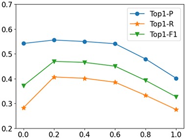
First, the biased item α is introduced to appropriately weigh observed and unobserved entries. The loss function is optimized only using positive samples when α = 0 and only using unobserved samples when α = 1. In this experiment, we fix|$L=3$|, |$K=3$| and|$H=2$|. Figure 3 shows the effects of different α on the prediction performance of NMR-RGCN. The performance when α = 0.2 is superior to the performances when α is set to be other values.
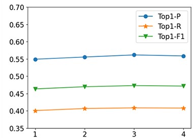
Second, we analyze the effect of |$L$| to the prediction performance. In this experiment, we fix|$\alpha =0.2$|, |$K=3$| and|$H=2$|. The comparative results are shown in Figure 4. From the results, we see that NMR-RGCN with |$L=3$| provides the best performance. Additionally, we also note that with L increasing (|$L>3$|), the performance of RGCN encoders slightly decreases as higher graph convolutional layers oversmoothed the encoded embeddings.
Finally, as described in the subsection Decoders score multicategory miRNA–disease association, the neural multirelational decoder consists of the local category-specific neural networks and the global neural networks across all categories. In the experiments, we fix |$\alpha =0.2$| and |$L=3$|. We test the following situations:
(1) Local linear decoder + global linear decoder. In this case, we only consider the linear local and global decoders, i.e. |$K=1$|, |$H=1$| and remove the nonlinear activation function. The results show that the performance of the linear decoder is far worse than that of the neural decoder.
(2) Local neural decoder. We remove the global decoder and only consider the local neural decoders. From the experimental results in Table 4, we found that the prediction performance of the model decreases when we removed the global decoder. It indicates that the global decoder is necessary for NMR-RGCN to improve the prediction performance.
(3) Local neural decoder + global neural decoder. We test the performance of several combinations of local neural decoders and global neural decoders. From the results in Table 4, we found that the prediction performance improved as the number of local neural decoder layers increases. However, when |$K>3$|, the prediction performance decreases slightly. Similarly, for the global neural projection, when |$H\le 2$|, the prediction performance improved as the number of layers increases. Note that the NMR decoder with |$K=3$| and |$H=2$| achieves the best performance.
Comparisons with existing work
Based on the above evaluation experimental results in the previous subsection, we use α = 0.2 |$, L=3,K=3$| and |$H=2$| as experimental settings for NMR-RGCN and α = 0.2|$, L=1, K=3$| and |$H=2$| for NMR-GCN in the comparison experiments. The learning rate of Adaptive Moment Estimation is 9e-4 and the regulation coefficient is 1e-8.
We have not found other approaches developed for predicting multiple categories of miRNA–disease associations except for only three methods [33–35]. Here, we compare NMR-RGCN (our method) with two methods: NLPMMDA [34], TDRC [35]. NLPMMDA predicted multirelational miRNA–disease associations by label propagation which integrates miRNA similarity and disease similarity. There are two hyperparameters in NLPMMDA, we set|${\lambda}_m=0.2$|, |${\lambda}_d=0.2$|, respectively as the original paper to get a best performance. TDRC introduced tensor decomposition with miRNA functional similarity and disease semantic similarity as relational constraints to solve the multiple types of miRNA–disease association prediction. There are four hyperparameters in TDRC, we set |$\lambda =0.001$|, |$\gamma =4$|, |$\alpha =0.125$| and |$\beta =0.25$|, respectively as the original paper to get a best performance. All compared experiments were carried on TDRC v3.2 dataset, TDRC v2.0 dataset and MCD-6 dataset, respectively.
We summarize the experimental comparison results of our proposed model and baselines on three datasets in Table 5. All experiments are evaluated under the two aforementioned experimental settings. We start by comparing the results in TDRC v2.0 and TDRC v3.2 datasets. We found that the improvements of NMR-RGCN, NMR-GCN and TDRC are particularly obvious compared with NLPMMDA, which highlights the importance of considering the relationship between each type of association. Then, we further compared NMR-RGCN with TDRC and NMR-GCN on the MCD-6 dataset. We observed that NMR-RGCN achieves relative performance gains over TDRC by 35.78% in terms of Top-1 precision and 1.51% in terms of AUC. This shows that capturing the nonlinear relationship between multiple types of miRNAs and diseases can enable us to obtain better results, because TDRC is essentially a multilinear method and may not be enough to capture the complex and nonlinear interactions between the features of miRNAs and diseases. When compared with NMR-GCN, the average relative Top-1 precision of NMR-RGCN is improved by 7.94%, because the proposed NMR-RGCN also takes into account heterogeneous information from other sources in the heterogeneous network when encoding node information.
Case studies
To further evaluate the accuracy of our proposed model for predicting unobserved miRNA–disease-type entries, we conduct case studies on two widespread human diseases, i.e. breast cancer and lung cancer (Supplementary Tables 3 and 4). We prioritized candidate miRNA-type pairs for a specific disease using the trained model based on MCD-4 dataset (all known HMDD v2.0 data), and then we verified the top-50 predictions with HMDD v3.2 dataset and recent literature. We also trained RGCN-NMR model based on MCD-6 dataset (all known HMDD v3.2 data), and then prioritized all unknown miRNA–disease-type entries using their predicted scores. Table 6 shows the top-10 predicted results and seven predictions can be confirmed according to recent literature. The results prove that our proposed model is effective.
The prediction and validation of top-10 miRNA–disease-category associations
| MiRNA | Disease | Categories | Evidence(PMID) |
|---|---|---|---|
| hsa-mir-34c | Carcinoma, hepatocellular | Epigenetics | 27165229 |
| hsa-mir-34a | Carcinoma, hepatocellular | Epigenetics | 27165229 |
| hsa-mir-21 | Multiple sclerosis | Other | Unconfirmed |
| hsa-mir-196a-2 | Ovarian neoplasms | Genetics | 30930933 |
| hsa-mir-126 | Breast neoplasms | Circulation | 20801493 |
| hsa-mir-21 | Leukemia, lymphoblastic, acute | Circulation | Unconfirmed |
| hsa-mir-21 | Alzheimer disease | Circulation | 31592314 |
| hsa-mir-146a | Osteosarcoma | Genetics | Unconfirmed |
| hsa-mir-155 | Bladder neoplasms | Tissue | 31298320 |
| hsa-mir-150 | Breast neoplasms | Circulation | 31963351 |
Conclusion
Identification of potential multicategory miRNA–disease associations using computational approaches is important as it will improve our understanding of the pathogenesis of diseases and guide treatment. In this study, we develop a novel data-driven end-to-end learning-based method NMCMDA of neural multiple-category miRNA–disease association prediction to deal with the issue of MCMDA. NMCMDA shows excellent performance for the prediction of multicategory miRNA–disease associations and is significantly superior to the state-of-the-art method TDRC [35] in terms of Top-1 precision, Top-1 Recall and Top-1 F1. In terms of our understanding, the advantages of NMCMDA over TDRC [35] may lie in the following two aspects. First, NMCMDA is an end-to-end learning framework where encoder operates directly on the miRNA–disease heterogeneous network and leverages GNN to learn latent representations. Decoder yields miRNA–disease association scores with the learned latent representations as input. All parameters involved in encoders and decoders are simultaneously optimized via a gradient descent. Although TDRC is not an end-to-end learning algorithm which cannot guarantee the latent feature is directly related to prediction objective. Second, TDRC is essentially a multilinear method and may not be enough to capture the complex and nonlinear interactions between the features of miRNAs and diseases. Case studies also provided for two high-risk human diseases breast cancer and lung cancer) and we also provide the prediction and validation of top-10 miRNA–disease-category associations based on all known data of HMDD v3.2, which further validate the effectiveness and feasibility of the proposed method.
There are several directions for future study. First, the structural information regarding miRNA and disease similarity networks significantly affects the learned feature representations, which further affects the final prediction results. Other sources of biomedical information, such as miRNA–gene interactions and disease–gene interactions, etc., might be relevant for modeling miRNA–disease associations, and we hope to investigate the utility of integrating them into the model. As our proposed NMCMDA is a general approach for multirelational link prediction in any heterogeneous network, it would be interesting to apply it to other domains and problems, for example, the identification of multirelational drug–drug interactions [43].
Present a novel data-driven end-to-end learning-based method of neural multiple-category miRNA–disease association prediction (NMCMDA) for predicting multiple-category miRNA–disease associations.
NMCMDA with the encoder of Relational Graph Convolutional Network and the neural multirelational decoder (NMR-RGCN) achieves the best prediction performance.
The experimental results show that the NMR-RGCN is significantly superior to the state-of-the-art method TDRC in terms of Top-1 precision, Top-1 Recall, and Top-1 F1.
Acknowledgements
We thank anonymous reviewers for valuable suggestions.
Funding
National Natural Science Foundation of China (U1802271), the Science Foundation for Distinguished Young Scholars of Yunnan Province (2019FJ011), the Fundamental Research Project of Yunnan Province (201901BB050052).
Jingru Wang is a postgraduate student at Yunnan University. Her research focuses on bioinformatics and machine learning.
Jin Li is currently a professor at the School of Software, Yunnan University. His research interests include bioinformatics and machine learning.
Kun Yue is currently a professor at the School of Information, Yunnan University. His research interests include data and knowledge engineering.
Li Wang is a postgraduate student at Yunnan University. Her research focuses on bioinformatics and graph data analysis.
Yuyun Ma is a postgraduate student at Yunnan University. Her research focuses on graph neural network.
Qing Li is an associate chief physician at the First Affiliated Hospital of Kunming Medical University. His research focuses on pathology.
