


Abstract
Biomolecular recognition between ligand and protein plays an essential role in drug discovery and development. However, it is extremely time and resource consuming to determine the protein–ligand binding affinity by experiments. At present, many computational methods have been proposed to predict binding affinity, most of which usually require protein 3D structures that are not often available. Therefore, new methods that can fully take advantage of sequence-level features are greatly needed to predict protein–ligand binding affinity and accelerate the drug discovery process. We developed a novel deep learning approach, named DeepDTAF, to predict the protein–ligand binding affinity. DeepDTAF was constructed by integrating local and global contextual features. More specifically, the protein-binding pocket, which possesses some special properties for directly binding the ligand, was firstly used as the local input feature for protein–ligand binding affinity prediction. Furthermore, dilated convolution was used to capture multiscale long-range interactions. We compared DeepDTAF with the recent state-of-art methods and analyzed the effectiveness of different parts of our model, the significant accuracy improvement showed that DeepDTAF was a reliable tool for affinity prediction. The resource codes and data are available at https: //github.com/KailiWang1/DeepDTAF.
Introduction
Biomolecular recognition plays a vital role in many biological processes, including immune targeting of non-self-protein, specificity of human catalytic kinases [1], etc. In general, proteins often act as targets and need to interact with ligand to regulate import biological functions in drug discovery [2, 3]. Previous researches also showed protein–ligand interactions are vital in mediating enzyme catalysis [4], signal transduction [5] and other biomolecule functions. And the disruption of their complexity is associated with some disease. The binding affinity can provide important information on the strength of protein–ligand interaction and is usually expressed by inhibition constant Ki, dissociation constant Kd or half-maximal inhibitory concentration IC50. The successful identification of affinity performs a crucial role in virtual screening of drug discovery and repurposing of existing drugs [6]. More specifically, the discovery of ligand binding targeted protein with high affinity is the major focus of early-stage drug research [7]. In protein–ligand interaction, the binding pocket is crucial for their interaction specificity. The p38 MAP kinase protein, for example, can form an allosteric binding pocket to regulate protein function by directly binding the compound. And the binding can induce a large conformation change that inhibits the kinase activity for treating some inflammatory [8]. Therefore, these studies suggest that local and global structural properties make important contribution to functions.
Researching the mechanisms of protein–ligand interactions is essential for drug development. However, it remains challenging to identifying the binding ligand from a large-scale chemical space through currently experimental methods [9], especially for protein or protein–ligand complex with unknown structures. Due to insufficient known structures of protein–ligand complexes [10] and time or resource consuming in the experiment, it is necessary to develop some computational methods to predict protein–ligand binding affinity. Some physics-based methods, such as molecular docking [11, 12], molecular dynamics (MD) simulations [13], have been popularly used in binding affinity prediction and virtual screening of small molecules interacting with proteins. These methods have good physical interpretability toward the interaction between molecules. However, these traditional structure-based methods still remain challenging for enormous computational resources consumption. Some similarity-based [14] or matrix factorization-based [15] methods give the prediction by using the global similarity matrices of entire proteins or ligands. The limitation of these methods is that the detailed features of individual components in each molecule are ignored. The support vector machines (SVM) and random forest (RF) algorithms [16, 17] for predicting protein–ligand interaction mostly focus on binary classification studies. As the accumulate of data and the development of artificial intelligence [18], the deep learning methods also become popular in affinity prediction, such as Pafnucy [19], DeepAtom [20] and the topological neural network TopologyNet [21]. These structure-based methods need detailed information for atoms of each molecule, while limiting to available high-quality protein–ligand complex structures. In order to overcome the structure-based limitation, some structure-free methods have been proposed. MONN [22] is the multi-objective model, which has more interpretability for the binding affinity prediction. However, it will take a long time for data preprocessing. DeepDTA [23] and WideDTA [24] are the models that rely on protein sequences and ligand SMILES as input, while ignoring more physiochemical information.
In this paper, we develop a novel deep-learning-based method, named DeepDTAF, to predict the protein–ligand binding affinity by integrating local and global features. More specially, the DeepDTAF comprises three separate modules, i.e. entire protein module, local pocket module and ligand SMILES module. And the input of each module is represented by residues of sequence or SMILES strings of compound. While the residue information of sequence contains not only the type, but also the structural properties, i.e. secondary structure elements, physicochemical characteristics. The protein and pocket modules are provided to extract global and local features, respectively. Dilated convolution and traditional convolution are used to capture both long-range and short-range interactions. The final features of the convolution and max pooling layers for the three modules are concatenated together and feed to classification part. In addition, we also tested our model on a database and compared with other competing models. These results suggested that DeepDTAF is a useful tool to provide the reliable prediction for protein–ligand binding affinity.
Materials and methods
Datasets
PDBbind database [25] includes a collection of experimentally verified protein–ligand binding affinity expressed with -logKi, -logKd or -logIC50 from the Protein Data Bank [10]. Here, we focused on three datasets in the PDBbind database version 2016 just as the previous computational methods did. The general set provides 9226 collected protein–ligand complexes. The refined set contains 4057 high-quality affinity data and complexes in total. And the core 2016 set was usually used as a high-quality benchmark, which included diversiform structures and binding data for evaluating various docking methods [26, 27]. To ensure there was no data overlap between these three datasets, the 290 protein–ligand complexes in the core 2016 set were removed from the refined set. Furthermore, for a convenient model comparison, 85 protein–ligand complexes in the validation set and 2 protein–ligand complexes in the training set were also removed to keep consistence with the Pafnucy. Finally, the general set included 9221 complexes, the refined set included 3685 complexes and the core 2016 set included 290 complexes. These datasets have provided protein PDB files, pocket PDB files and ligand SDF files, etc. Here, we collected the protein sequence, pocket sequence according to the PDB files. And the SDF files were converted to SMILES strings. In our model, considering that the 3D structures of some proteins are still unknown, we only used the 1D sequence data to provide input information. Moreover, due to the different lengths of protein sequences, pocket sequences and SMILES strings, it is necessary to ensure fixed lengths in order to create an effective representation form. The fixed lengths for protein sequences, pocket sequences and SMILES strings were chosen, respectively, based on the distributions illustrated in Figure 1. The maximum length of protein, ligand and pocket sequence is 4720, 472 and 125, respectively. Therefore, we defined the fixed 1000 characters for protein sequences, 150 characters for SMILES strings and 63 characters for pocket sequences to cover around 90% of proteins, 90% of ligands and 90% of pockets in these datasets. The sequences that are longer than the fixed characters were truncated and the sequences that are shorter than the fixed characters were 0 padded.
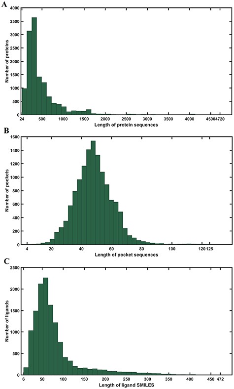
Statistics of lengths of all data in the study. (A) Distribution of lengths of protein sequences. The maximum and minimum lengths are 4720 and 24, respectively. (B) Distribution of lengths of pocket sequences. The maximum and minimum lengths are 472 and 6, respectively. (C) Distribution of lengths of ligand SMILES. The maximum and minimum lengths are 125 and 4, respectively.
Here, we used the same method of Pafnucy [19] to split training set and validation set. Thousand randomly selected complexes in the refined set were used as validation set. The remaining 11 906 complexes of the refined set and the general set were used as the training set. Additionally, the core 2016 set was compiled to test and evaluate our model. The Smith–Waterman similarity [28] for each protein sequence in the core 2016 test set was at most 60% [23] to any sequence in the training set for 99% of protein pairs. Furthermore, in order to give a more objective evaluation, we collected another two test sets from the Protein Data Bank [10]. One of the test sets included 105 data (test105) and the Smith-Waterman similarity for each protein sequence was at most 60% to any sequence in the training set. Another test set had 71 data (test71) and the sequence identity was smaller than 35% [29, 30] to the sequences in the training set. And the test sets are listed in Supplementary Table S1. The distributions of affinity values for the core 2016 set, test105 set, test71 set and all data were presented in Supplementary Figure S1.
Input representation
In this study, only 1D sequence data were used by label encoding, the 3D structures of proteins, ligands or their complexes were not included in the input representation. To obtain the interaction information more effectively, we divided the text-based input information into three parts, ligand representation, protein representation and pocket representation. In most of the previous work, the input representations of protein sequence and ligand SMILES were showed to be effective to predict the protein–ligand binding affinity [23]. Here, we have added additional pieces of input information, likely structural property information and binding pocket information, which proved to be beneficial for affinity prediction. The details of the input information are listed as follows.
Ligand representation
The popular 1D representation for ligand chemical structure was Simplified Molecular Input Line Entry System (SMILES) [31] based on atoms, bonds, rings, etc. Here, we used Open Babel [32] to convert all of ligand SDF files into the SMILES strings. Sixty-four characters were used for the representation of ligand SMILES strings. Each character was encoded by a special integer (e.g. ‘H’: 12, ‘N’: 14, ‘C’: 42, ‘O’: 48, ‘(’: 1, etc.). The example of encoding SMILES strings is showed as |$[C\ C\ C\ C\ (=O\ )\ C]=[42\ 42\ 42\ 42\ 1\ 40\ 48\ 31\ 42]$|
Protein representation
Sequence representation
Amino acid is the component of protein sequence. And most protein sequences usually consist of 20 different types of amino acids. Besides, the non-standard residues are also included in some proteins. Here, we used a 21D one-hot vector to encode 21 different types of residues in protein sequence.
Structural property representation
Considering the experimentally solved protein structures is still insufficient and the structure prediction without templates remains a challenge, we thus use protein structural properties as alternative features. The protein structural properties are well available and could provide more abundant information [33, 34]. In this study, the structural properties included secondary structure elements (SSEs) [35, 36] and physicochemical characteristics. Here, we used SSPro program [37] to predict secondary structure for each sequence. The eight categories of secondary structure states included α-helix (H), residue in isolated β-bridge (B), extended strand, participates in β ladder (E), hydrogen bonded turn (T), 310 helix (G), π-helix (I), bend (S) and coil (C) [38]. We used an 8D one-hot vector to encode SSEs. Furthermore, non-polar, polar, acidic, basic [39] based on structure of side chain and seven groups according to their dipoles and side chain volumes [40, 41] (see Supplementary Table S2) for each residue were provided to describe physicochemical characteristics. Therefore, 11D vector was used to encode physicochemical characteristics. Taken together, 19D vector for each residue was used to represent structural property.
In summary, we used a 40D feature vector for each residue to describe global protein features by integrating sequence and structural property representation.
Pocket representation
The pocket usually means a binding cavity in the interior or on the surface of the protein, which possesses some special physicochemical and geometric properties to directly bind small compound. In fact, the amino acids of the pocket define specific physicochemical properties, which combine with the shape and location of the pocket to determine protein functions. Furthermore, the protein–ligand interaction mainly depends on the binding between ligand and protein pocket [42]. And the pocket is componented by a discontinuous sequence including some key amino acids of protein. Therefore, a pocket is regard as the whole for local features extraction. The local pocket features are crucial and are firstly used as input information in protein–ligand binding affinity prediction. Here, a 40D feature vector for each residue of pocket was used to encode local pocket features by integrating sequence representation and structural property representation described in above subsection.
Model
Model construction
In this study, the deep convolutional neural network-based architecture [43] was applied to DeepDTAF for predicting the binding affinity. The prediction model was proposed to deal with a regression problem by using the following procedures (Figure 2). The input feature has been described in the previous section. Here, we used embedding layer to represent inputs with 128D dense vectors in three modules. The embedding layer was applied to transform a sparse vector to a denser vector by feeding integer encoded inputs. So these modules consisted of (1000, 128), (63, 128, 150, 128) dimensional matrices for protein, pocket and ligand, respectively. More specifically, for protein module, the 1D dilated convolution [44] with five different dilated rates was used considering the long-range interactions of longer protein sequence. The dilated convolution layers were then followed by the max pooling layer, which was same as ligand module. However, the dilated convolution included four different dilated rates in ligand module. In order to illustrate the difference of dilated convolution between the two modules, dilated convolution A and B were used to distinguish them in the procedures. For pocket module, we used three 1D traditional convolutions with increasing number of filters. So, the convolutional layers consisted of 32, 64, 128 filters, and the size of filter was 3. Then, the max pooling layer followed. Finally, the features of the max pooling layers for the three modules were concatenated together and fed to the classification part. The classification part consisted of three fully connected (FC) layers. The first FC layer had 128 nodes and the second FC layer had 64 nodes. Each layer was followed by the dropout layer of rate 0.5. The dropout layer stochastically set some activations of hidden units to zero for fighting against over-fitting [45]. The last FC layer was followed by the output layer.
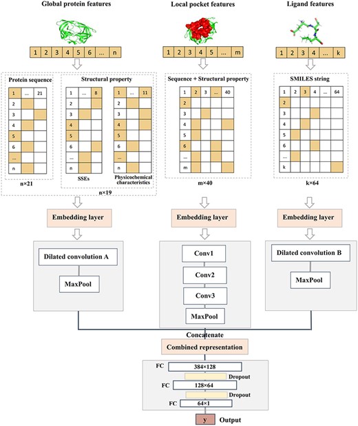
Architecture of DeepDTAF. DeepDTAF first transforms 1D sequences of protein, pocket and ligand into sequence, structural property information or SMILES information, then feeds the input information to embedding layer and dilated or traditional convolution layers. Finally, these features are concatenated and feed into FC layers for binding affinity prediction.
In summary, we developed a model that combined the local and global features for extracting more abundant interaction information, and the dilated convolution was used to replace traditional convolution for enlarging the receptive field and capturing more long-range interactions.
Local and global feature
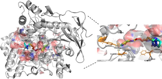
From the biological point of view, the key amino acids and their interactions derived from local sequences are generally considered important. However, in previous deep-learning based model study, the global features derived from entire protein sequences have been used for predicting protein–ligand binding affinity, while, the local features are often ignored [23]. Indeed, in many biological processes, the protein pockets play an essential role as targets and directly bind small molecule. Such as, the inhibitor binding pocket of HIV-1 protease (PDB code: 1G2K) [48] is recognized as an attractive target for antiviral treatment. In this study, the interactions between binding pocket of 1G2K and inhibitor are shown in Figure 3 and Supplementary Table S3. Here, the interactions are calculated by LIGPLOT program [49]. Furthermore, besides the residues involving in the binding pocket, the other residues of sequence also play important roles in the protein functions and some long-range interactions with ligand. The sequence of amino acids specifies a protein’s structure and range of motion, which in turn determine its function. Therefore, the global features representing the whole protein sequence are important in this study. Overall, the local and global properties are critical to protein function and complex interaction. Here, the deep learning model was constructed to capture the importance of different input positions by integrating the local and global features for protein-binding pocket sequences and entire protein sequences.
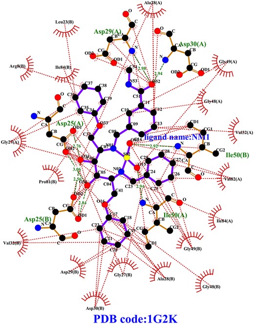
Diagram of 2D ligand-pocket interaction for 1G2K. The ligand bonds and ligand name NM1 are colored in purple. The hydrophobic residue of pocket and hydrophobic interactions between pocket residues and ligand are colored in red. The hydrogen bonds between residues and ligand are indicated by the green dotted lines. The hydrogen bond residues are colored in yellow and the names are colored in green.
Dilated convolution
Here, dilated convolution was used to capture long-range interactions for protein features and ligand SMILES by increasing the effective receptive field size. The protein module had 5 layers that apply 3 |$\times$|3 convolutional kernels with different dilation rates of 1, 2, 4, 8, 16. The ligand module had four layers that apply 3 |$\times$|3 convolutional kernels with different dilation rates of 1, 2, 4, 8.
Evaluation metrics
Results and discussion
In this study, the deep learning-based model was introduced to predict the protein–ligand binding affinity. DeepDTAF model incorporated up to three text-based input information modules: the global protein module, the local pocket module and the ligand SMILES module. In fact, our model was constructed by combining the local and global features. Furthermore, the dilated convolution was also used in our model to capture multiscale information and more long-range interactions. The results showed that DeepDTAF given more accurate prediction than other competing methods. Moreover, we tested the effectiveness of different parts of our model architecture. The local pocket features, which contain more direct and detailed information for binding affinity determination, are proved to be the most useful information in the architecture.
Comparison with competing methods
Here, training was carried out for 20 epochs, the model with lowest error in validation set was selected. Furthermore, to evaluate the performance of DeepDTAF in predicting protein–ligand binding affinity, we compare DeepDTAF with three state of the art deep learning models, DeepDTA [23], Pafnucy [19] and TopologyNet [21]. DeepDTA is a traditional 1D convolutional neural network prediction model that includes primary sequences (1D representations) of proteins and SMILES strings of ligands without adding additional pieces of input information. Pafnucy is a deep neural network model that utilizes a 3D convolution to produce a feature map of the protein–ligand 3D structure. We recalculated the predicted affinity by the DeepDTA and Pafnucy model for 11 906 protein–ligand data in training set, 1000 data in validation set, 290 data in core 2016 test set and 105 data in test105 set. The downloaded DeepDTA program and Pafnucy program are used to analyze protein–ligand data. TopologyNet is a structure-based model by integrating the element-specific persistent homology (ESPH) method and deep convolutional neural networks. ESPH is the method that represents 3D complex geometry via 1D topological invariants. We calculated the predicted affinity for core 2016 test set and test105 set by using TopologyNet. The TopologyNet is the online software (https://weilab.math.msu.edu/TDL/TDL-BP/index.php) for protein–ligand affinity prediction. As expected, DeepDTAF can provide good performances in the two test sets, which were unknown during model training and validation. As shown in Table 1 and Figure 4, the performance of DeepDTAF was evaluated on the PDBbind database. In fact, we found that DeepDTAF could provide better performance than other competing methods on the core 2016 test set (Table 2 and Figure 5). RMSE (1.355) in DeepDTAF, as one of the metrics of prediction error, is lower than DeepDTA (RMSE = 1.443), Pafnucy (RMSE = 1.418), TopolopyNet (RMSE = 3.713). The correlation R of 0.789 in DeepDTAF is improved 4.0% (DeepDTA), 1.4% (Pafnucy) and 61.6% (TopologyNet), the CI of 0.799 was improved 2.8% (DeepDTA), 1.0% (Pafnucy) and 24.4% (TopologyNet). The other metrics in DeepDTAF, such as MAE and SD, also outperformed DeepDTA, Pafnucy, and TopologyNet. Furthermore, DeepDTAF was more accurate as compared with other competing methods on test105 set (Table 3 and Figure 6). Despite 60% sequence similarity, the 35% sequence similarity was also analyzed in the test71 dataset. And the values of RMSE, MAE, R, SD, CI were showed in Table 4 and Figure 7. The results showed that our model performed better in affinity prediction.
Performance of DeepDTAF
| Datasets | RMSE | MAE | R | SD | CI |
|---|---|---|---|---|---|
| Test | 1.355 | 1.073 | 0.789 | 1.337 | 0.799 |
| Validation | 1.367 | 1.054 | 0.747 | 1.365 | 0.779 |
| Training | 0.952 | 0.731 | 0.864 | 0.942 | 0.839 |
| Datasets | RMSE | MAE | R | SD | CI |
|---|---|---|---|---|---|
| Test | 1.355 | 1.073 | 0.789 | 1.337 | 0.799 |
| Validation | 1.367 | 1.054 | 0.747 | 1.365 | 0.779 |
| Training | 0.952 | 0.731 | 0.864 | 0.942 | 0.839 |
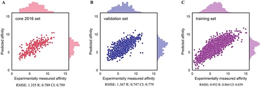
Distributions of predicted affinities on core 2016 test set (A), validation set (B) and training set (C) for DeepDTAF.
Predictions accuracies of DeepDTAF and other competing methods on core 2016 test set
| Methods | RMSE | MAE | R | SD | CI |
|---|---|---|---|---|---|
| DeepDTA | 1.443 | 1.148 | 0.749 | 1.445 | 0.771 |
| Pafnucy | 1.418 | 1.129 | 0.775 | 1.375 | 0.789 |
| DeepDTAF | 1.355 | 1.073 | 0.789 | 1.337 | 0.799 |
| TopologyNet | 3.713 | 3.151 | 0.173 | 2.142 | 0.555 |
| Methods | RMSE | MAE | R | SD | CI |
|---|---|---|---|---|---|
| DeepDTA | 1.443 | 1.148 | 0.749 | 1.445 | 0.771 |
| Pafnucy | 1.418 | 1.129 | 0.775 | 1.375 | 0.789 |
| DeepDTAF | 1.355 | 1.073 | 0.789 | 1.337 | 0.799 |
| TopologyNet | 3.713 | 3.151 | 0.173 | 2.142 | 0.555 |
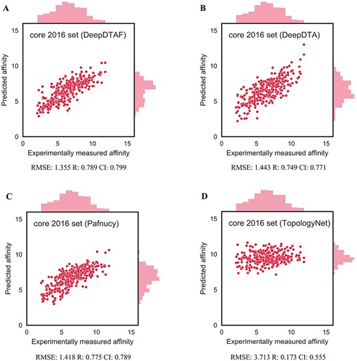
The performance of DeepDTAF (A), DeepDTA (B), Pafnucy (C) and TopologyNet (D) on core 2016 test set for the prediction of binding affinity.
Predictions accuracies of DeepDTAF and other competing methods on test105 set
| Methods | RMSE | MAE | R | SD | CI |
|---|---|---|---|---|---|
| DeepDTA | 1.425 | 1.134 | 0.652 | 1.432 | 0.738 |
| Pafnucy | 1.392 | 1.169 | 0.750 | 1.176 | 0.782 |
| DeepDTAF | 1.247 | 0.966 | 0.766 | 1.149 | 0.801 |
| TopologyNet | 4.143 | 3.841 | 0.444 | 1.530 | 0.646 |
| Methods | RMSE | MAE | R | SD | CI |
|---|---|---|---|---|---|
| DeepDTA | 1.425 | 1.134 | 0.652 | 1.432 | 0.738 |
| Pafnucy | 1.392 | 1.169 | 0.750 | 1.176 | 0.782 |
| DeepDTAF | 1.247 | 0.966 | 0.766 | 1.149 | 0.801 |
| TopologyNet | 4.143 | 3.841 | 0.444 | 1.530 | 0.646 |
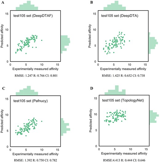
The performance of DeepDTAF (A), DeepDTA (B), Pafnucy (C) and TopologyNet (D) on the test105 set for the prediction of binding affinity.
Predictions accuracies of DeepDTAF and other competing methods on test71 set
| Methods | RMSE | MAE | R | SD | CI |
|---|---|---|---|---|---|
| DeepDTA | 1.517 | 1.144 | 0.417 | 1.527 | 0.641 |
| Pafnucy | 1.442 | 1.210 | 0.427 | 1.230 | 0.628 |
| DeepDTAF | 1.273 | 0.998 | 0.480 | 1.194 | 0.656 |
| TopologyNet | 4.157 | 3.913 | 0.192 | 1.308 | 0.559 |
| Methods | RMSE | MAE | R | SD | CI |
|---|---|---|---|---|---|
| DeepDTA | 1.517 | 1.144 | 0.417 | 1.527 | 0.641 |
| Pafnucy | 1.442 | 1.210 | 0.427 | 1.230 | 0.628 |
| DeepDTAF | 1.273 | 0.998 | 0.480 | 1.194 | 0.656 |
| TopologyNet | 4.157 | 3.913 | 0.192 | 1.308 | 0.559 |
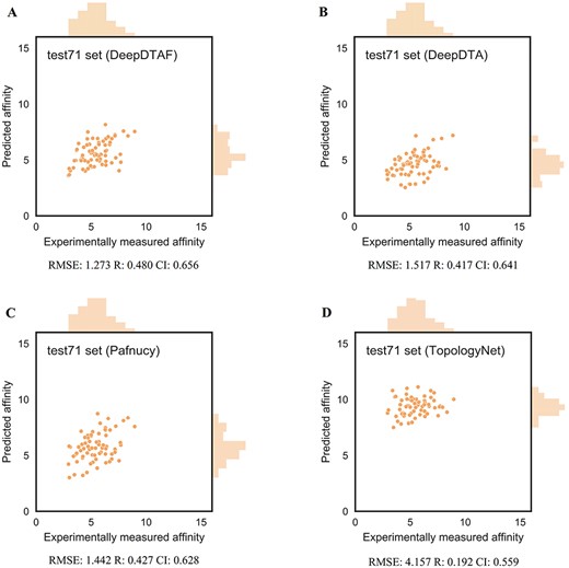
The performance of DeepDTAF (A), DeepDTA (B), Pafnucy (C) and TopologyNet (D) on the test71 set for the prediction of binding affinity.
The effects of local pocket features
The binding pocket possesses some special properties for directly binding ligand to define the function. More specifically, some binding sites are located on the concave surfaces of the protein. In the process of biomolecular recognition, the small molecule will bind to the binding sites to form a special conformation to perform its function. For example, acetylcholinesterase (PDB code: 1H22) binding ligand inhibitor was often applied in the treatment of Alzheimer’s disease (AD) [54]. The crystal complex structure of acetylcholinesterase with inhibitor is shown in Figure 8. PyMOL is used to analyze the hydrogen bonds and visualize the protein–ligand structure and the putative cavity. And in our test set, the predicted affinity for protein 1H22 is 9.18, which is very close to the experimentally measured affinity value 9.10. Briefly, the protein binding pockets are crucial for the protein–ligand interactions and usually used as targets for disease treatment.
Cartoon representation of acetylcholinesterase (PDB code: 1H22) binding ligand inhibitor E10. The hydrogen bonds between pocket and ligand are showed in the enlarged figure. The ligand is represented by sticks and colored in rainbow, the pocket is represented by surface and colored in blend, and the protein is colored in gray. The yellow dotted line denotes the hydrogen bonds between ligand and binding pocket. The residues of the pocket that interact with ligand are colored in orange.
Here, the protein-binding pocket as local features was considered to be the critically important information for protein–ligand binding affinity prediction. Therefore, we tested the effects of local pocket features. Firstly, we trained our model based on the raw data sets but removing local pocket features extraction module. The performance of our model without local pocket features on core 2016 test set is shown in Table 5, all evaluation metrics were clearly worse than raw DeepDTAF model. Such as, it achieved a decrease in R by up to 5.7% compared with raw model. Furthermore, the model without global protein features was also tested and resulted in worse performance. Taken together, these results indicate that we can get better performance by combining local pocket features and global protein features. And the large drop of evaluation metrics indicates that local pocket features include extremely important information for protein–ligand binding affinity prediction.
Predictive accuracies of DeepDTAF and DeepDTAF without local features, physicochemical characters, SSEs, dilated convolution on test set
| Models | RMSE | MAE | R | SD | CI |
|---|---|---|---|---|---|
| Without local features | 1.518 | 1.268 | 0.732 | 1.482 | 0.767 |
| Without physicochemical characters | 1.404 | 1.118 | 0.767 | 1.396 | 0.783 |
| Without dilated convolution | 1.403 | 1.134 | 0.775 | 1.376 | 0.788 |
| Without SSEs | 1.338 | 1.112 | 0.781 | 1.360 | 0.790 |
| DeepDTAF | 1.355 | 1.073 | 0.789 | 1.337 | 0.799 |
The effects of different types of structural properties
In this study, besides the raw protein sequence information, the structural property information of protein and pocket was also used in the model. The structural properties included SSEs and physicochemical characteristics. Protein SSEs and physicochemical characteristics of amino acids are important toward the function characterization. In order to study the effects of different types of structural properties in DeepDTAF, we conducted an ablation research by removing the SSEs, physicochemical characteristics, respectively. As shown in Table 5, the structural properties, specially the physicochemical characteristics play essential roles for identifying protein–ligand binding affinity. Furthermore, to validate the effectiveness of fixed input lengths, we also compared the 90% length cutoff in our model with 80% cutoff, 85% cutoff, 95% cutoff and 100% cutoff. Our results showed the 90% cutoff is the best (Supplementary Figure S2).
Comparison between predicted SSEs and real SSEs
We studied the accuracy of the predicted secondary structure and its influences on results. As stated in the original article [37], the accuracy of SSpro rose to 92.9%. It has been known that the prediction of SSEs is relatively mature. So, the predicted secondary structure for each sequence was used as the input information in our model. Furthermore, we also used DSSP program [38] to generate real secondary structure. We applied the real SSEs to replace the predicted SSEs in our model for affinity prediction. Figure 8 displayed the results of our model and the model with real SSEs on the core 2016 test set. The RMSE of DeepDTAF with real SSEs is 1.340 (DeepDTAF: 1.355), CI of DeepDTAF with real SSEs is 0.797 (DeepDTAF: 0.799), R of DeepDTAF with real SSEs is 0.792 (DeepDTAF: 0.789). Furthermore, MAE of DeepDTAF with real SSEs is 1.059 (DeepDTAF: 1.073), SD with real SSEs is 1.329 (DeepDTAF: 1.337). From the results, we can obtain that the accuracy of the model with predicted SSEs and the model with real SSEs is similar. Thus, it is reasonable to use the predicted SSEs as the input features in our model (Figure 9).
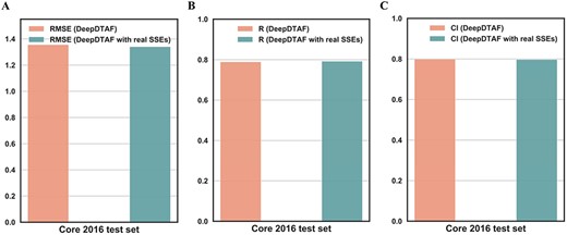
The values of RMSE (A), CI (B), R (C) for DeepDTAF and DeepDTAF with real SSEs on the core 2016 test set.
The effects of dilated convolution
Dilated convolution was used to increase the effective receptive filed size and capture multiscale contextual information. Compared with traditional convolution, the advantage of dilated convolution is that it can capture multiscale long-range interactions between amino acid residues for long contextual sequences. In this paper, we used dilated convolution in protein and ligand modules for more accurate prediction. Furthermore, to prove the importance of dilated convolution, we tested the model by replacing dilated convolution with traditional convolution (Table 5). It is summarized that the dilated convolution could provide better performance for the prediction.
Affinity analysis with binding pocket
The pocket plays a vital role in protein–ligand interaction. Here, besides the features used in our model, the pocket volume and pocket hydrogen bond were also analyzed in affinity prediction. We randomly selected 30 proteins in the core 2016 test set for pocket volume and hydrogen bond acceptors computation (Figure 10). It is interesting to note that there is a correlation between affinity values (Figure 10A) and pocket volumes (Figure 10C) with the correlation coefficient of 0.692. And a correlation coefficient between affinity values (Figure 10A) and number of hydrogen bond acceptors in pocket (Figure 10D) is 0.667. The results suggested that pocket volume and hydrogen bond acceptors were useful information for affinity prediction. In the future, more pocket features will be considered to optimize our model. Similarly, we found that the correlation coefficient between predicted affinity values (Figure 10B) and pocket volumes (Figure 10C) is 0.596, and the correlation coefficient between predicted affinity values (Figure 10B) and number of hydrogen bond acceptors (Figure 10D) is 0.524. The results showed that although the whole pocket features, such as pocket volumes and number of hydrogen bond acceptors, were not explicitly incorporated into our model, some related information could still be captured by DeepDTAF.
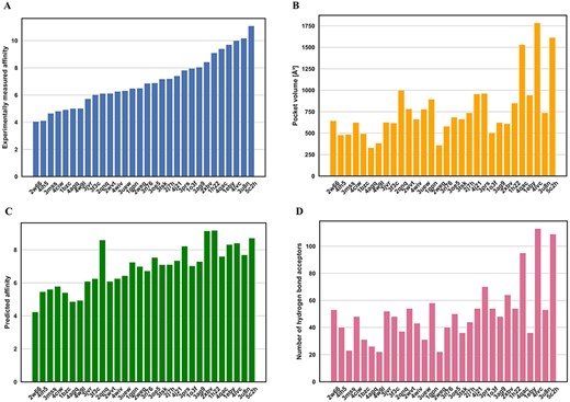
Relation between affinity value (A and B) and pocket volumes (C) and number of hydrogen bond acceptors (D) for 30 proteins in the core 2016 test set. The predicted affinities are generated by DeepDTAF.
Conclusion
For protein–ligand binding affinity prediction, the current DeepDTA algorithm only use sequences of proteins and ligands without other physicochemical characteristics. The Pafnucy and TopologyNet algorithms are based on protein–ligand complex 3D structures. However, this method is limited to known complex structures. In this study, we developed the deep learning-based approach DeepDTAF for predicting binding affinity. DeepDTAF distinguished itself from the competing algorithms in the follow aspects. Firstly, we integrated the local and global features of proteins for extracting information of different scales. Secondly, besides the protein sequence feature, we added additional structural properties for proteins, i.e. SSEs and physicochemical characteristics, which possess more biological significance. Thirdly, dilated convolution was constructed in the entire protein and ligand modules to capture multiscale long-range interactions. We also tested the effects of these new features, the results indicated that they were useful for the affinity prediction. When compared with other competing methods, our model has the better performance for binding affinity prediction.
In the process of protein ligand recognition, the short-range binding pocket and long-range allosteric effect can provide useful information for function characterization and protein–ligand interaction. Furthermore, the SSEs and physicochemical characteristics of residues also have a crucial impact on function. Taken together, the DeepDTAF comprises three separate modules, i.e. entire protein module, local pocket module and ligand SMILES module. The residue types, SSEs and some physicochemical characteristics can be obtained from 1D sequence. Thus, we used them as the input information of protein and pocket modules. Then, dilated convolution was used to extract long-range interactions from the protein and ligand modules. And traditional convolution was used to capture short-range interactions from the pocket module. Finally, the three modules were fed into FC layers together to predict binding affinity. Though DeepDTAF is demonstrated to have better results compared with other competing methods, it also has some limitations. The present architecture relies on the types of training data, so it may be better to provide larger training data. Another one is that our approach includes single information for ligand module. In the future, we will optimize the ligand module for capturing more important features. Moreover, the shape and location of pocket also should be considered to improve the prediction.
In this study, we constructed a new deep learning architecture, DeepDTAF, which was used to capture short-range and long-range interactions by combining the local and global features. Some correlative results showed that DeepDTAF was a reliable tool for predicting protein–ligand binding affinity.
A novel deep learning-based architecture by integrating local and global features was developed and applied for protein–ligand binding affinity prediction.
The protein-binding pocket was first used as the local input feature in the model to predict protein–ligand binding affinity.
DeepDTAF was an effective method that combined the dilated convolution with traditional convolution to capture multiscale interactions for protein–ligand binding affinity prediction.
Funding
The National Natural Science Foundation of China (grant no. 61832019); Hunan Provincial Science and Technology Program (2019CB1007); the Degree & Postgraduate Education Reform Project of Hunan Province (No. 2019JGYB051); and the Fundamental Research Funds for the Central Universities, CSU (2282019SYLB004).
Kaili Wang received the M.S. degree in college of physical science and technology from Central China Normal University, China, in 2019. Currently, she is working toward the Ph.D. degree in computer science in the Central South University, Changsha, China. Her current research interests include bioinformatics, deep learning and drug-target research.
Renyi Zhou received the B.S. degree in computer science from Central South University, Changsha, China, in 2020. He is a master at the School of Computer Science and Engineering, Central South University. His current research interests include bioinformatics and deep learning.
Yaohang Li is an associate professor in the Department of Computer Science at Old Dominion University, Norfolk, USA. His current research interests are in computational biology, Monte Carlo methods, big data analysis and parallel/distributed/grid computing.
Min Li received the B.S. degree in communication engineering and the M.S. and Ph.D. degrees in computer science from Central South University, Changsha, China, in 2001, 2004 and 2008, respectively. She is currently a professor at the School of Computer Science and Engineering, Central South University. Her main research interests include bioinformatics and system biology.
Reference
Author notes
Kaili Wang and Renyi Zhou contributed equally to this work and as first authors.
