


Abstract
RNA-binding protein (RBP) is a class of proteins that bind to and accompany RNAs in regulating biological processes. An RBP may have multiple target RNAs, and its aberrant expression can cause multiple diseases. Methods have been designed to predict whether a specific RBP can bind to an RNA and the position of the binding site using binary classification model. However, most of the existing methods do not take into account the binding similarity and correlation between different RBPs. While methods employing multiple labels and Long Short Term Memory Network (LSTM) are proposed to consider binding similarity between different RBPs, the accuracy remains low due to insufficient feature learning and multi-label learning on RNA sequences. In response to this challenge, the concept of RNA-RBP Binding Network (RRBN) is proposed in this paper to provide theoretical support for multi-label learning to identify RBPs that can bind to RNAs. It is experimentally shown that the RRBN information can significantly improve the prediction of unknown RNA−RBP interactions. To further improve the prediction accuracy, we present the novel computational method iDeepMV which integrates multi-view deep learning technology under the multi-label learning framework. iDeepMV first extracts data from the views of amino acid sequence and dipeptide component based on the RNA sequences as the original view. Deep neural network models are then designed for the respective views to perform deep feature learning. The extracted deep features are fed into multi-label classifiers which are trained with the RNA−RBP interaction information for the three views. Finally, a voting mechanism is designed to make comprehensive decision on the results of the multi-label classifiers. Our experimental results show that the prediction performance of iDeepMV, which combines multi-view deep feature learning models with RNA−RBP interaction information, is significantly better than that of the state-of-the-art methods. iDeepMV is freely available at http://www.csbio.sjtu.edu.cn/bioinf/iDeepMV for academic use. The code is freely available at http://github.com/uchihayht/iDeepMV.
Introduction
To perform its function smoothly, RNA usually needs to be mediated by an RNA-binding protein (RBP). It may fail to perform regulatory or translational function due to deregulated-RBP. RBP also plays a key role in post-transcriptional events. The versatility and structural flexibility of their RNA-binding domains allow RBPs to control the metabolism of a large number of transcriptions. There are approximately 1542 human RBPs identified, accounting for 7.5% of all proteins encoded by gene. They are involved in almost all steps of the post-transcriptional regulatory layer. With RBPs, highly dynamic interactions with other proteins and RNAs are established, e.g. regulating RNA splicing, polyadenylation, stabilizing, positioning, translation and degradation [1,2]. Studies have found that RBP is dysregulated in cancer [3]. Therefore, deciphering the intricate and interconnected relationship between RBPs and the cancer-related RNA targets can provide a better understanding of tumor biology and insights into new cancer treatments [4]. As most RNAs can bind to more than one RBP [5], finding RBPs with similar binding capacity has become an important research direction.
Machine learning is a promising approach that has been widely exploited to identify RBP’s binding sites from RNA sequences [6]. For example, Maticzka et al. [7] proposed the GraphProt method to learn the binding preference of RBP’s sequences and structures from high-throughput experimental data. Corrado et al. [8] proposed a method called RNACommender, which was able to recommend RNA targets to unexplored RBPs through the available interaction information by taking into account the protein structure and the predicted secondary structure of RNAs. The beRBP model, proposed by Yu et al. [9], trained random forest models to predict the RNA targets for general and specific RBPs using the motif information. The existing machine learning based methods mainly focus on the use of the sequence or structural characteristics of the original RNA sequence to predict the binding site [10,11].
Recently, deep learning has achieved remarkable success in computational biology, including RNA-protein interaction prediction. The method DeepBind [12] applied Convolutional Neural Network (CNN) to learn the binding preference of individual RBPs and achieved superior performance. Pan et al. [13] proposed the iDeepE method using a global CNN model to predict the binding site of RNA and RBP by studying the RNA sequence. They further considered unique combination structures of RBPs [14] and proposed the iDeepS method to learn the binding preference of the sequences and structures simultaneously. iDeepS employed two separate CNNs and a Long Short Term Memory Network (LSTM) to capture the sequences and structural motifs of the RBP-binding sites [15]. The two methods above trained RBP-specific models that were designed separately for each RBP, and they could only predict the binding of RNAs to a specific RBP with a large number of verified binding RNAs. In addition, the strategy did not consider the shared binding similarity among different RBPs. To resolve the above issues, Pan et al. [16] further proposed a new method called iDeepM, which used multi-label classification and deep learning to identify multiple RBPs that can interact with an RNA. However, iDeepM also has the shortcomings. First, it is not clear whether the RNA−RBP interaction information is helpful to predict new interactions. Furthermore, there exist many types of RBPs but the feature learning network of iDeepM is rather simple, therefore the prediction accuracy is still low and needs further improvement.
To address the issues of iDeepM, this study proposes the iDeepMV method which integrates the technologies of multi-view feature learning, deep feature learning and multi-label classification technology for RBP recognition. First, based on the raw RNA sequences, we extract data for the amino acid sequence view and the dipeptide component view. Then, with the multi-view data, we design deep neural network models of the respective views to learn the deep features, which are used to train multi-label classifiers that can effectively exploit the correlation between the labels. Finally, a voting mechanism is used to further improve the prediction accuracy by yielding a decision that is made by considering the results of each view comprehensively. Our experimental results show that with the multi-view deep feature learning models combined with the RNA−RBP interaction information, the prediction accuracy of iDeepMV is highly competitive when compared to the state-of-the-art methods.
The main contributions of this paper can be summarized as follows: (i) We confirm that the existing RNA−RBP interaction information is helpful to improve the prediction of RNA−RBP interactions; (ii) By encoding the text sequences, we propose a new method to convert RNA sequences into amino acid sequences; (iii) Features of the RNA sequence from three views are extracted to establish the corresponding deep neural network model to further extract the deep features; (iv) Multi-label classifier is applied to learn the associations between RNAs and RBPs. The trained classifier can predict which RBPs that an unexplored RNA can bind to; (v) The impact of the number of samples on the performance of the model is identified.
The article is organized as follows. In Section 2, we introduce in detail the auxiliary experiments conducted to verify the effectiveness of RNA-RBP Binding Network (RRBN) for predicting binding, and the working principle of iDeepMV. Comparative test and results in Section 3 show the advantages of our method in identifying the accuracy of RBPs. In Section 4, we make a summary and discussion of the work, and funds that support our work are given in Section 5.
Materials and Methods
Overview
iDeepMV formulates the identification of the binding between RBPs with an unexplored RNA as a multi-label classification problem. Here, RNA sequence is regarded as research subject, and RBPs are used as labels. Different from the existing methods, we convert the original RNA sequence into amino acid sequence and dipeptide components according to the principle of molecular biology, and obtain the initial data of the RNA view, amino acid view and dipeptide view, respectively. Deep CNN is then applied to extract the deep features from the initial data of these three views. Next, the Classifier Chains (CC) model is used as multi-label classifier to learn the correlation between the labels. The classifier trained by the CC model predicts which RBPs that an unexplored RNA can bind to. Finally, a voting mechanism is designed to combine the results from the three views to determine the final prediction result. The overall framework of iDeepMV is illustrated in Figure 1. iDeepMV consists of four modules: initial multi-view data, deep multi-view feature learning, multi-label classifier training and multi-view voting.
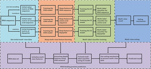
Overall framework of iDeepMV. First, an RNA sequence is sent to the data processing module to get the initial data of the three views, which are then fed into the CNN models to extract the respective deep features. Next, the deep features are used to train the multi-label classifiers to obtain the preliminary prediction. The voting module makes the final decision based on the results of the three classifiers.
Besides, the data flow of the experiment is depicted in Figure 2. It shows how the raw data are processed through our model to obtain the final results. First, the raw text data are extracted from the dataset, and the data of the other two views are then separated by multi-view data processing. The one-hot encoding technique is used to process the text data to produce the input data for the CNN model. Next, the CNN model generates deep features as the input data of the downstream CC classifiers. The preliminary classification results of each view are then obtained using the CC classifiers. Finally, the classification results of the three views are integrated using the voting mechanism to get the final results.
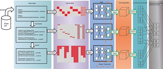
The data flow in the experiment: raw data extracted from the dataset undergoes the processes of data encoding, CNN network model, multi-label classification and voting to obtain the prediction results.
RNA-RBP binding network
The data used in this paper are obtained from the AURA website [17]. It is a manually compiled database of human untranslated regions (UTRs) and UTR regulators. AURA integrates RNA sequence and structure data, regulatory and mutation sites, gene and protein expression and gene function descriptions from scientific literature. We obtain 137 003 RNA sequences, 1264 regulatory factors and 2549 510 binding sites between them. Regulatory factors, also known as trans-acting factors, are a class of protein regulatory factors encoded by the genes upstream of the transcription template, including activating factors and repressors. Common regulatory factors are RBP, miRNA and transcription factors. We only select the data related to RBPs, and finally adopt 67 RBPs, 73 681 RNA sequences and 550 386 binding sites between them, as shown in Figure 3.
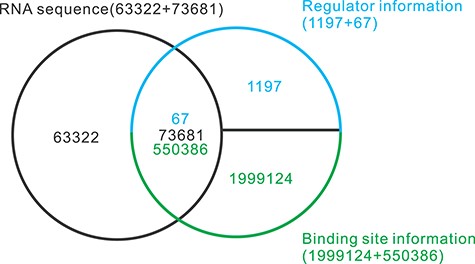
Selection of data from the AURA database. Sixty-seven RBPs, 73 681 RNA sequences and the 550 386 binding sites between them are used in the study. In addition, 18 421 RNA sequences without any binding sites are added into the benchmarking dataset as negative samples.
In nature, one RNA can bind to multiple RBPs, and one RBP can also bind to multiple RNAs. This forms an intricate network of binding relationships between them, which is referred to as RRBN in this paper. Investigation of the underlying laws of this network can provide significant assistance in predicting new RNA−RBP interactions. We introduce the related concepts of graph theory [18] to quantify the RNA-RBP network in two dimensions. With the data selected above, a 0–1 matrix of size 73 681 × 67 (corresponding to 73 681 RNAs and 67 RBPs) as shown in Table 1 is obtained, which is called the RNA-RBP Binding Matrix (RRBM).
The RRBM constructed with 73 681 RNAs and 67 RBPs
| ADAR1 | AGO1 | AGO2 | AGO4 | ALKBH5 | ATXN2 | C17ORF85 | |
|---|---|---|---|---|---|---|---|
| uc001aeo.2_3UTR | 1 | 1 | 0 | 0 | 0 | 0 | 0 |
| uc001aer.3_3UTR | 1 | 1 | 0 | 0 | 0 | 1 | 0 |
| uc001aeu.1_3UTR | 1 | 1 | 0 | 0 | 0 | 1 | 0 |
| uc001amu.2_5UTR | 1 | 0 | 1 | 0 | 0 | 1 | 0 |
| uc003pkv.2_3UTR | 0 | 1 | 1 | 0 | 1 | 1 | 1 |
Prediction of new RNA−RBP interactions with existing binding information
In order to investigate whether the existing binding information of an RNA to some RBPs can help predict new RNA−RBP interactions, we conduct experimental analysis using the RNA sequence information in AURA database and the RRBM.
First, given an RNA sequence, we transform it into a vector α with the rule ‘A = 2, C = 3, G = 4, U = 5’. Then, the binding information of this RNA, with 66 kinds of RBPs in the RRBM, is concatenated with α to give the new vector β. In addition to these 66 RBPs, the 67th RBP-binding information of this RNA is used as the label value y to compare with the predicted value y’. For comparison, we use α and β as the input samples to train a classifier in machine learning to predict label y’. For the 73 681 sample data, we divide it into a training set and a test set at the ratio of 4:1. The training set is inputted to the machine learning algorithm for training. The trained model predicts the result of the test set, which is compared with the true label values to evaluate the accuracy of the model.
Since the binding information of each of the 67 RBPs is highly imbalanced, 67 sets of experiments are conducted such that in each experiment the binding information of an RBP is used as the label value y, whereas the other binding information is taken as the components of the vector β. For experiments that use the vector α as the input sample, only y is taken as the label value. To our knowledge, this is the first time that the effectiveness of RRBN in predicting RNA−RBP interactions is investigated, and therefore baseline models are not available for comparison. Hence, in this study, we select four popular machine learning algorithms to build models for investigating the effectiveness of RRBN. These algorithms include Support Vector Machine (SVM) [19,20], BP Neural Network [21], Decision Tree [22] and Random Forest [23,24]. The details are given in Part A of the Supplementary Material.
Extraction of multiple-view features
Most existing methods that use multi-modal data of RNA sequences to build models for predicting the binding sites of RBPs on RNAs mainly focus on the sequences and structures. The models are trained, respectively, with the data of each modality and the final prediction is the combination of the outputs from the individual models. To better integrate multi-view data (RNA sequence view, amino acid view and dipeptide component view), the proposed iDeepMV uses multi-view extraction techniques to transform the initial RNA sequence into more informative multi-modal data. At the same time, we design a unique training model for the data of each view and extract the deep features to learn the relevance of the labels.
RNA sequence encoding
RNA sequence is a text sequence of four alphabets. The text sequence is encoded as a numerical matrix which is fed into a machine learning model. Considering that the length of the RNA sequences in the dataset is not uniform and CNN can only process data of the same size, we specify a fixed length of 2700 and base B as a temporary base that is added to complement the length of each RNA sequence. One-hot encoding [25] is currently the most popular encoding technology. It is used to construct an initial 4 × m one-hot encoded matrix for an RNA sequence of length m, as shown in Part B of the Supplementary Material .
Amino acid sequence constructing
Although the RNA’s one-hot encoded matrix is informative for predicting RNA−RBP interactions, it ignores the context information. To incorporate context information and retain more sequence feature, RNA sequences are first converted into higher-dimensional amino acid sequences [26]. Since RNA sequence has a stop codon, and some RNA sequences contain a temporary base B, we use the letter O to represent them during the conversion. As the transformation of an RNA sequence into an amino acid sequence is unidirectional and unique, one amino acid can correspond to multiple base combinations. Thus, the resulting amino acid sequence cannot be converted back to the original RNA sequence, which could result in information loss. For example, the base combination ‘GCA’ can be transformed into a specific amino acid A, but the amino acid A can also be converted from ‘GCC’, ‘GCG’ or ‘GCU’.
To solve the problem, iDeepMV involves three forms of translation: (1) transcode from the beginning, (2) skip the first base to start transcoding and (3) skip the first and the second bases to start transcoding. An RNA sequence of length m is converted into three amino acid sequences of length 1/3 × m. Amino acid sequences transformed into these three forms can restore the original RNA sequence by complementing the sequence information. For example, for the sequence fragment ‘CGCAU’, we can get the amino acids R, A and H corresponding to the three morphological sequences. Since amino acids R and A have the same base ‘GC’, and amino acids A and H have the same base ‘CA’, we can uniquely determine that the base combination is ‘GCA’. Therefore, by concatenating the three amino acid sequences to produce a long chain of amino acids with length m, the sequence information of the original RNA sequence can be fully restored. Similar to RNA sequence, an initial feature matrix of size 20 × m can be obtained, as shown in Part C of the Supplementary Material.
Dipeptide component statistics
The RNA sequence view and the amino acid view are biased toward the features extracted from the sequence order. In addition to sequence order, sequence components also contain important information. For example, dipeptides are widely used to investigate the structure of an amino acid sequence component [27]. G-gap dipeptide composition [28] is a method used for describing the composition of dipeptides in amino acid sequences.
The g-gap dipeptide method maps the amino acid sequence to a feature vector, where ‘g’ is a parameter that represents a dipeptide with a gap of ‘g’ amino acids in between and the value ranges from 0 to 9. In this study, we test the performance of 10 kinds of g-gap dipeptide models using the same dataset and select 0-gap dipeptide as our research subject. The results are listed in Part D of the Supplementary Material. Due to the spatial structure of amino acids, dipeptides are sensitive to the arrangement of the left and right amino acids [29,30]. Thus, for the 21 amino acids (20 amino acids and one temporary amino acid O), there are 441 dipeptide combinations. With the combination ‘OO’ discarded, 440 dipeptides are taken into account. The different appearances of each dipeptide constitute the feature vectors, which can effectively capture the component information and the amino acid arrangement information. Furthermore, we convert the 440-D vector into a two-dimensional histogram, as shown in Part E of the Supplementary Material, to extract the depth features more effectively.
Extraction of high-level features using CNN
Based on the initial data obtained from the three views, we construct three different deep CNN models which are trained separately to obtain high-level features. CNN performs powerful representation learning and translation-invariant classification according to the hierarchical structure in the data [31–33]. There are three types of layers in the CNN models, i.e. convolution, pooling and full connection layer. The convolution kernel in the convolution layer contains weight coefficients while the pooling layer does not have any learnable parameters. In this study, the CNN models constructed for the three views are similar.
Figure 4 shows the CNN model and illustrates the extraction of high-level features for each view. The expression k @ m × n represents the number k and size (m × n) of the feature maps in each layer of the network. The input of the entire model is the encoded data matrix of each view. As a result, a 68-dimensional feature vector is obtained, corresponding to 68 class (67 types of RBP and a class that is unrelated to any of the 67 RBPs). The activation function used in the last layer of the CNN is the sigmoid function. Note that the last layer of the network is just to ensure the model fit the outputs. In our study, the main purpose of CNN is to extract effective high-level features to train the downstream multi-label classifier. For a trained CNN, the penultimate layer usually contains more discriminant information than the output layer. So we take the concatenated 202-dimensional features of the penultimate layer as the extracted deep features, which will be used for training the downstream multi-label classifier.
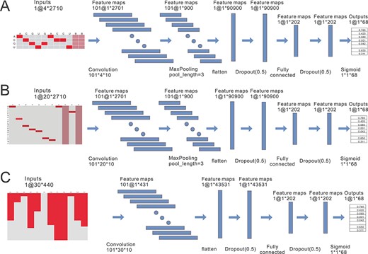
Extracting high-level features from the three views using deep CNN models. (A) The CNN model is used to extract the high-level features of the RNA sequence. It contains a convolutional layer, a pooling layer and two fully connected layers. One-hot coding encodes the RNA sequence into a (4 × 2700) matrix. Note that the size of the input layer matrix in (A) is 4 × 2710. This is because when one-hot encoding is used for conversion, we artificially add five blank cells to the head and tail of the sequence, so that the length of the feature map generated after one convolution can be exactly divided in the pooling layer. From the input layer to the convolutional layer, we use 101 convolution kernels of size 20 × 10, with a step size of 1, to obtain 101 (1 × 2701) feature maps, which are then down-sampled by the maximum pool to obtain 101 (1 × 900) feature maps. The 101 feature maps are further flattened to obtain a 90 900-dimensional feature vector. Next, in order to prevent over fitting, a dropout operation is performed, followed by the first fully connected operation to compress the feature vectors obtained from the previous layer into 202-dimensional feature vectors. Finally, the output layer is a 68-dimensional fully connected layer activated by the sigmoid function. (B) The CNN model is used to extract the high-level features for the amino acid sequence. As in (A), the model is also composed of four network layers, a convolutional layer, a pooling layer and two full connected layers. (C) Similarly, CNN model is used for deep feature extraction of the dipeptide component. Since the size of the initial feature matrix of the dipeptide component is 30 × 440, which is relatively small, the max-pooling layer is abandoned in the CNN model.
In the three models shown in Figure 4, except for the last fully connected layer where the sigmoid activation function is used, the activation functions of the other network layers are relu. This is because the relu function is computationally more efficient that can prevent the gradient from disappearing to some extent.
Multi-label classifier training
This study aims to identify the RBPs that an unexplored RNA can bind to. This can be formulated as a multi-label classification problem. There are mainly two approaches of multi-label classification. The first approach is problem conversion method that combines multiple labels into a certain form to obtain a label set, which is regarded as a special label to indirectly convert the problem into a single-label learning problem. Classical algorithms of this approach include BR [34], LP [35] and CC [36]. The BR algorithm designs several classifiers to effectively learn the features of each class but ignoring the correlation between the labels. The LP algorithm considers the connection between the labels, but the time and space complexity of the algorithm is relatively high. The CC algorithm uses multiple classifiers to construct a chain structure, which can effectively learn the intricate relationships between the labels. The other approach is to adapt the existing single-label learning method for multi-label classification. The widely used algorithms are Boosting-based AdaBoost.MH (AMH) and AdaBoost.MR (AMR) [37], and decision tree based methods. AMH uses the Hamming Loss Function to build a learning model whereas AMR uses the Ranking Loss Function. Clare et al. [38] improved the classical single-label decision tree and proposed the C4.5 algorithm. The principle is to train the classifier by calculating the information gain of the training samples. In the improved algorithm, the leaf node is no longer a class, but a label set.
By analyzing the characteristics of the different methods discussed above, this paper adopts the CC model as the multi-label classifier after extracting the deep features, in which the RNA interacting RBPs are the labels. The CC multi-label classifier used in this paper is to construct a classifier chain based on binary classification to learn the association between the labels. The principle is illustrated in Figure 5. In this experiment, the CC multi-label classifier consists of 68 binary classifiers, which are used to predict the corresponding 68 labels. First, we obtain the 202-dimensional depth feature from the upstream CNN model, and use it as the input feature to start training the first binary classifier. The first label value predicted by the first classifier is appended to the 202-dimensional deep feature, which is to be used as the input feature of the second binary classifier to continue the training. The process repeats until the last classifier is trained. The CC multi-label classifier can learn the association between the labels because each time when a sub-classifier is trained, the predicted label value is added to the initial feature for the next round of training, which establishes relationships with the 68 independent classifiers. The algorithm of CC is detailed in Part F of the Supplementary Material. We train the respective CC multi-label classifiers using the high-level features extracted from the three views. The obtained multi-view results are combined to obtain the final prediction results through the voting mechanism in the downstream.
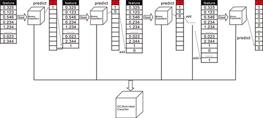
The principle of CC multi-label classifier. After each round of classifier training, the predicted label value is added as a new feature for the next round of training, which is how CC multi-label classifier learns the association between the labels.
Multi-view and multi-label voting mechanism
Voting mechanism is a combination strategy to integrate the results of multiple classifiers [39]. The basic idea is to simply count the predictions obtained by all multi-view machine learning algorithms and the final result is the one with the highest count, i.e. majority vote.
The classifier can directly give the final prediction label or the prediction probability of the output label. The former is called majority or hard voting; the latter is called soft voting. Hard voting counts the prediction value (say, 0 or 1) of each method and the final result is given by the one with the highest count. Soft voting combines the prediction probability of each method to calculate the weighted sum of the probability, and finally determines whether the prediction result is 0 or 1 according to a predefined threshold. In this paper, hard voting is adopted, and the weights of the three views are set to be equal by default.
Results
Following the methods described above, experiments were conducted from three aspects: (1) to demonstrate the power of the existing binding information of RNAs and RBPs for predicting the new RNA−RBP interactions; (2) to evaluate the performance of the proposed iDeepMV in predicting the RBPs that an unexplored RNA can bind to; and (3) to compare iDeepMV with the state-of-the-art iDeepM method and the variants of iDeepMV. The results are given as follows.
Existing binding information has a certain effect on prediction
In order to demonstrate that the existing binding information of RNAs and RBPs is useful for predicting new RNA−RBP interactions, we constructed an RNA sequence vector α without binding information, an RNA sequence vector β with binding information and 67 types of RBP as the labels, respectively. The prediction models SVM, BP Neural Network, Decision Tree and Random Forest were trained. The performance was evaluated on the 67 RBPs in terms of accuracy, precision and recall. The results of 5-fold cross-validation are shown in Figure 6. In the figure, SVMα and SVMβ denote SVM trained with RNA sequence vector α and β, respectively. Similar notations are used for the other prediction models. It can be seen that the models trained with β outperformed those with α, demonstrating that the existing binding information of RNA and RBP is helpful for predicting new RNA−RBP interactions. The accuracy of most models is above 90%, but the precision and recall are quite different. This is because negative samples are the majority in the benchmark dataset, and therefore it is more meaningful to refer to precision and recall.
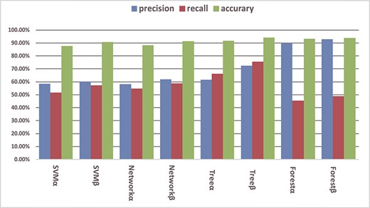
The effect of binding information on RBP prediction performance in terms of accuracy, precision and recall. The average results of five-fold cross-validation using four prediction models are given, with and without the use of binding information as indicated by α and β, respectively.
Among the four prediction models, decision tree and random forest exhibit better performance. This is because the input vectors and labels of the experiments are integers which fit the settings of these two models. Decision tress is indeed the best model for predicting new RNA−RBP interactions with the existing binding information using the RRBN. The precision and recall are 72.47% and 75.66%, respectively.
The amount of RBP-RNA binding information has a big impact on predicting new RBP−RNA interactions
In the auxiliary experiment, we used the data in the RRBM to construct the binding information of the vector β. Note that in the RRBM, only the number ‘1’ is the binding information that we have confirmed, and we call it a positive sample. The number ‘0’ does not mean that the corresponding RNA and RBP cannot be combined, but the dataset does not have their binding information. There are two possibilities: they can be combined and cannot be combined. Because of the uncertainty, it cannot be regarded as a real negative sample in that sense. So we only analyze the impact of positive samples in this experiment.
To study the effect of the amount of positive samples in the RBP-binding information on the prediction of new RNA−RBP interactions, we used the RNA sequence vector β with binding information as input data, trained 100 decision trees and obtained 100 sets of results. As shown in Figure 7, the classes with a small number of positive samples have a lower precision, which indicates that the model fails to learn their features for the minority classes. As the number of positive samples in the classes increases, the RNA sequence information and binding information are enriched, and the prediction performance is improved gradually and steadily. However, the prediction accuracy does not strictly increase with the increase in the number of samples, some RBP prediction results even show large deviations, such as TNRC6B, U2AF2, etc. This may be due to the fact that some information of these classes that should be combined has not been exploited, resulting in positive samples being treated as negative samples and producing a completely opposite effect on model training, and eventually leading to significant reduction in prediction accuracy for these classes. The same phenomenon also occurs when the number of positive samples of a class is small and the impact of noises and error information on model learning is large. This is because in the prediction of these classes, the model tends to regard the positive samples as negative classes to reduce training loss which is reflected in the figure that the precision is falsely high, while the recall is low.
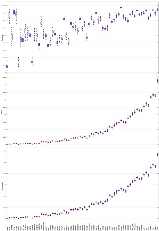
The impact of the number of positive samples on the precision, recall and F1-score (weighted sum of precision and recall) of the decision tree models. The abscissa are the types of RBP which are arranged in increasing order of the number of positive samples.
iDeepMV is superior to state-of-the-art method
We compared the performance of iDeepM and two variants of the proposed iDeepMV, i.e. iDeepMV− and iDeepMV+, under the benchmarking dataset constructed. Here, iDeepMV− refers iDeepMV without the multi-label classifier training phase, whereas iDeepMV+ includes the training phase. The results of 5-fold cross-validation are shown in Table 2. A comparison of the single-view and multi-view effects is shown in Figure 8.
Performance of RBP recognition: iDeepMV+ and iDeepMV− denote iDeepMV with and without using multi-label learning, respectively. For the three views, the plus sign appended to a view denotes a model trained using CNN and multi-label learning simultaneously using the data of that view, whereas the minus sign appended denotes a model trained using CNN only using the data of that view. For multi-view voting, the plus and minus sign appended indicate, respectively, that voting is applied on the results obtained from all the three views, with models trained using CNN and multi-label learning simultaneously and using CNN only
| Model | Macro-AUC | Micro-AUC | Weighted-AUC | Macro-F1 | Micro-F1 | Weighted-F1 | |
|---|---|---|---|---|---|---|---|
| iDeepM | 0.90 | 0.94 | 0.91 | 0.42 | 0.62 | 0.60 | |
| iDeepMV− | RNA view - | 0.92 | 0.95 | 0.93 | 0.70 | 0.74 | 0.74 |
| amino acid view - | 0.93 | 0.96 | 0.93 | 0.72 | 0.75 | 0.75 | |
| dipeptide view - | 0.95 | 0.97 | 0.95 | 0.71 | 0.75 | 0.75 | |
| Multi-view voting - | 0.73 | 0.77 | 0.77 | ||||
| iDeepMV+ | RNA view + | 0.90 | 0.94 | 0.91 | 0.75 | 0.77 | 0.77 |
| amino acid view + | 0.90 | 0.94 | 0.91 | 0.76 | 0.78 | 0.78 | |
| dipeptide view + | 0.94 | 0.96 | 0.94 | 0.75 | 0.79 | 0.78 | |
| Multi-view voting + | 0.78 | 0.80 | 0.80 | ||||
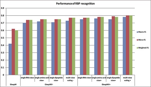
Histogram of performance comparison between single-view and multi-view models. Regardless of whether a multi-label classifier is used, the performance of the multi-view model is always better than that of the single-view model.
In the table, AUC is the area under the ROC curve. The ROC curve is a comprehensive indicator reflecting the continuous change of sensitivity and specificity [40]. The larger the AUC value, the better the classification performance. Due to class imbalance, the metrics Macro-AUC, Micro-AUC and Weighted-AUC are introduced. Macro-AUC is obtained by setting the same weight for each class, and summing the AUC of each class to calculate the average value. Micro-AUC is obtained by summing the sensitivity and specificity of each class separately, and representing the result as a ROC curve to get the AUC. Weighted-AUC is obtained by calculating the weight of each class according to the number of samples of each class to get the weighted sum of the AUCs of these classes. In addition, we calculate the F1-score which is the harmonic average of precision and recall. Similar to AUC, we also calculate Macro-F1, Micro-F1 and Weight-F1 accordingly. Since the voting mechanism have already integrated the voting results under the optimal threshold for each view, it is not necessary to consider the AUC for the voting results, which does not exist indeed.
It can be seen from the table that the AUCs of iDeepM and that of the three views proposed in this paper are close. The AUCs under the three restrictions are also not significantly different. However, the three F1 metrics of iDeepM are quite different, where Macro-F1 is much lower than Micro-F1 and Weighted-F1. This is because iDeepM has a small learning bias. After optimizing the network structure and learning the best classification threshold, we can see that iDeepMV exhibits a significant increase in the AUC and F1. The performance under the amino acid and dipeptide views are superior to that under the RNA view. The result demonstrates that the features extracted directly from the RNA sequences are not as informative as those extracted from the amino acid sequences and dipeptides. By integrating the results from the three views using the voting mechanism, the performance are further improved, indicating that the information of the three views can complement with each other.
Furthermore, the AUCs of iDeepMV+ under the three views are slightly lower than that of iDeepMV−, indicating that the performance of the CC multi-label classifier is inferior to the sigmoid layer in CNN for multi-label classification. However, the CC multi-label classifier integrates the information of the RRBN, resulting in higher accuracy, which demonstrates the association information between the labels can assist in predicting the RNP−RNA interactions. In summary, the experimental results show that by integrating deep learning model and multi-label classifier, the proposed iDeepMV can accurately identify the RBPs that an unexplored RNA can bind to.
The performance of iDeepMV is closely related to the amount of available binding information
For each RBP, we further evaluated the precision, recall and F1-score of iDeepM, iDeepMV+ and iDeepMV−. The detailed results are reported in Part G of the Supplementary Material. The performance change of the three methods with the different number of training samples is shown in Figure 9. The horizontal axis is the number of samples of the 67 RBPs which sorted in ascending order.
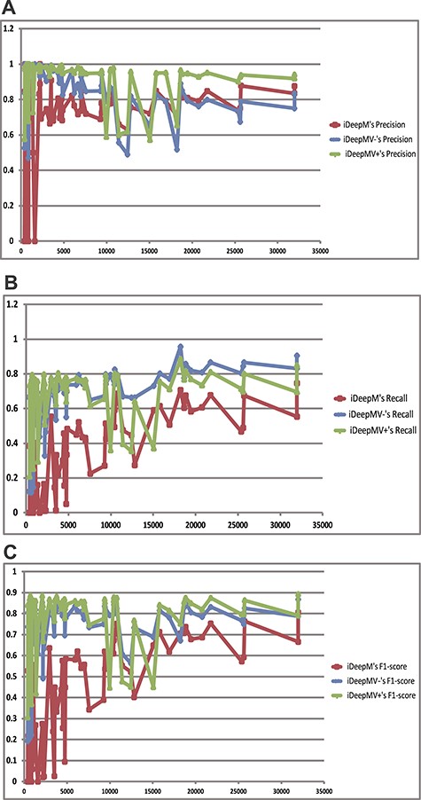
The performance change of iDeepMV with the number of training samples. iDeepMV− refers to iDeepMV without training by multi-label classifier, and iDeepMV+ refers to iDeepMV trained by multi-label classifier. (A) Precision; (B) Recall; (C) F1-score.
As shown in Figure 9, we can see that the performance of the two variants of iDeepMV increases with the number of training samples. When the number of samples is less than 5000, the change in the three metrics is very large. It is because the number of samples for some classes is too few that the deep learning model cannot learn the high-level characteristics for these classes. Besides, the learning ability of iDeepM is not as good as that of iDeepMV when the number of training samples is relatively few. The iDeepMV+ method with multi-label classifiers performs better than iDeepMV− and iDeepM. It has the best precision and F1, which are objective metrics for imbalanced data. With increasing number of samples for each class, the performance of iDeepMV is improved with a large margin as compared to iDeepM.
Conclusion and Discussion
Conventional classification methods usually train an RBP-specific model for each RBP to predict whether an RNA can interact with an RBP of interest. In this study, we focus on the prediction of the RBPs that can bind to specific RNA sequences, where the concept of RRBN is proposed for the first time. We have demonstrated that the RRBN can improve the prediction of new RNA−RBP interactions. Based on this conclusion, the multi-modal data of RNA sequence and the additional combined network information are used to establish a multi-view deep convolutional network model and a multi-label classifier for predicting the RNA interacting RBPs. Our results show that the proposed iDeepMV that is based on multi-view deep learning and multi-label learning achieves superior performance to the existing methods. We further demonstrate that it is beneficial to convert RNA sequences into amino acid sequences for feature extraction, and the features extracted from the dipeptide components of amino acids are also helpful for classification. In addition, the multi-label classifier based on the CC multi-label learning technology can learn the association between the labels, resulting in a better prediction performance. The decision obtained by synthesizing multiple views is comprehensive and further improves the prediction accuracy.
Despite the promising performance of iDeepMV, there are rooms for further improvement. For example, while iDeepMV trains the classifiers of each view independently, the model can indeed be trained on the three views collectively to further improve the prediction accuracy using multi-view learning techniques [41–44]. In addition, many multimodal data and methods applied to predict RBP-binding sites have achieved very good performance, such as sequence semantics and 4-order sequence combination coding. Although the use of these methods in the construction of RNA multimodal initial data may have a certain effect on interpretability of the models, it is still worthwhile to exploit them to further enhance the prediction accuracy.
Using the secondary structure of RNA or amino acid sequences as a new view for this study will theoretically improve the prediction performance. However, the prediction of the structure of long sequences is a very time-consuming task, which is particularly challenging for the 73 681 sequences with an average length of 2700 considered in this study. Meanwhile, class imbalance is a typical issue for the datasets concerned. How to use efficient methods to predict the structure of long sequences and construct a more suitable RBP recognition method for imbalanced data will also be important research directions.
The existing RNA and RNA-binding protein (RBP) interaction information is confirmed to be helpful to improve the prediction of RNA-RBP interactions.
In addition to the raw RNA sequence view, data for the amino acid sequence view and the dipeptide component view are also extracted, where deep features are learned from the three views by deep convolutional neural networks to predict the respective RNARBP interactions. It is demonstrated experimentally that the features extracted from the amino acid sequences and dipeptides are more informative than that from the RNA sequences.
Multi-label classifiers trained by the three views’ deep features are used to learn the associations between RNAs and RBPs. The trained classifier can predict the RBPs that an unexplored RNA can bind to.
The results conclude that the richer the combinations of RBP information, the more accurate the prediction of the unknown RNA-RBP interactions.
Funding
National Natural Science Foundation of China (61772239); Jiangnan University State Key Laboratory of Food Science and Technology Free Exploration Project under Grant (SKLF-ZZB-201901); The National First-Class Discipline Program of Light Industry Technology and Engineering (LITE2018–02 and LITE2018–03); The Six Talent Peaks Project in Jiangsu Province (XYDXX-056); The Jiangsu Province Natural Science Fund (BK20181339); The Innovation and Technology Fund of the Hong Kong Special Administrative Region of the People’s Republic of China (MRF/015/18); the National Natural Science Foundation of China (No. 61903248, 61725302, 61671288); RGC GRF project PolyU (512006/19E); Shanghai Municipal Science and Technology Major Project (No. 2018SHZDZX01).
Conflict of interest
The authors declare that there is no conflict of interests regarding the publication of this article.
Haitao Yang is a master student at Jiangnan University. His research interests include text data mining, natural language processing and their applications in bioinformatics.
Dr. Zhaohong Deng is a full-time professor in the School of Artificial Intelligence and Computer Science of Jiangnan University, Key Laboratory of Computational Neuroscience and Brain-Inspired Intelligence (LCNBI) and ZJLab. His research interests include bioinformatics, pattern recognition, computational intelligence and their applications.
Dr. Xiaoyong Pan is an assistant professor in the Department of Automation of Shanghai Jiao Tong University. His research interests include pattern recognition, image processing and data mining in bioinformatics.
Dr. Hong-Bin Shen is a full-time professor at Shanghai Jiao Tong University. His research interests include basic theory of pattern recognition and artificial intelligence, protein engineering and complex network in bioinformatics.
Dr. Kup-Sze Choi is a full-time professor at the Hong Kong Polytechnic University. His research interests include pattern recognition, data mining and image processing.
Dr. Lei Wang is a postdoctoral fellow of School of Biotechnology and Key Laboratory of Industrial Biotechnology Ministry in Jiangnan University. His research interests include enzyme fermentation engineering and food science.
Dr. Shitong Wang is a full-time professor in the School of Artificial Intelligence and Computer Science of Jiangnan University. His research interests include pattern recognition, computer application and light industry information technology.
Dr. Jing Wu is a full-time professor in School of Biotechnology and Key Laboratory of Industrial Biotechnology Ministry in Jiangnan University. Her research interests include the location of enzyme-encoded genes, the construction of high-efficiency expression systems for genetic engineering, the protein engineering of enzyme preparations and the genetic engineering of metabolic engineering strains.
