


Abstract
High-throughput data generated by new biotechnologies require specific and adapted statistical treatment in order to be efficiently used in biological studies. In this article, we propose a powerful framework to manage and analyse multi-omics heterogeneous data to carry out an integrative analysis. We have illustrated this using the mixOmics package for R software as it specifically addresses data integration issues. Our work also aims at applying the most recent functionalities of mixOmics to real datasets. Although multi-block integrative methodologies exist, we hope to encourage a more widespread use of such approaches in an operational framework by biologists. We have used natural populations of the model plant Arabidopsis thaliana in this work, but the framework proposed is not limited to this plant and can be deployed whatever the organisms of interest and the biological question may be. Four omics datasets (phenomics, metabolomics, cell wall proteomics and transcriptomics) were collected, analysed and integrated to study the cell wall plasticity of plants exposed to sub-optimal temperature growth conditions. The methodologies presented here start from basic univariate statistics leading to multi-block integration analysis. We have also highlighted the fact that each method, either unsupervised or supervised, is associated with one biological issue. Using this powerful framework enabled us to arrive at novel conclusions on the biological system, which would not have been possible using standard statistical approaches.
Introduction
Measurements used in the study of biological processes are becoming increasingly complex, and currently, biologists use a plethora of new technologies to elucidate the behaviour of biological systems. High-throughput measurements have revolutionized how we analyse the behaviour of organisms and predict, for example, their response to environmental changes. Today, each biological experiment can lead to the generation of large amount of data of different types, such as genome sequences, gene and protein expression levels, metabolite profiles and phenotypic observations. High-throughput technologies have also undergone revolutionary changes, which has had the result of greatly reducing the cost of omics data production. This, in turn, opens up new possibilities for the development of effective tools for data treatment and analysis [1].
Heterogeneous data collected at different levels from cellular to organism level are associated with a wide variety of techniques. Data acquisition therefore requires a suitable methodology [2] and a specific experimental design since an experimental design that is inadequate for an integrative analysis could complicate the final interpretation of the collected data. This point of view has been previously stated in Ref. [3] for microarray studies as follows: ‘While a good design does not guarantee a successful experiment, a suitably bad design guarantees a failed experiment—no results or incorrect results’.
Using multi-omics data enables to obtain a deeper understanding of the biological system under investigation [4, 5]. Quantification of data leads to improved accuracy and thus has great potential for finding answers to new questions. However, this revolutionary technique must be used with care since it is known, for instance, that it can be difficult to correlate transcriptomics and proteomics data [6–8]. Each of these technologies has its own limitations, and thus, collecting different types of data should help to understand the influence of one or more experimental conditions on the results. Thus, biological candidates can be identified as biomarkers under complex environmental conditions, and/or new complex regulations can be found.
Overall, it has been generally acknowledged that the analysis of a single kind of omics data is not sufficient to understand the effects of a particular treatment on a complex biological system. To obtain a holistic view, it is therefore preferable to combine multiple omics analyses [9].
This article proposes to link the development of statistical methodology to the investigation of biological systems and is expected to be of interest to scientists involved in multi-omics data analysis even when having little or no expertise in the application of statistical methods. We present a powerful framework to manage and analyse heterogeneous datasets acquired on a particular sample. Our methodology consists in progressing stepwise from basic univariate statistics to multi-block integration analysis [10, 11]. Regarding multivariate unsupervised analyses, we focus on projection-based methods and do not consider clustering approaches such as those described in Refs. [12–14]. We showcase here the improvements of each method starting from the computation of univariate statistics to a thorough implementation of multi-block exploratory analysis on the end result. The implementation of the methods chosen as well as the graphical representations have been achieved by adapting existing programs for the R software [15] and the mixOmics package [16]. However, it is generally not obvious to draw conclusions on the biological system by simply looking at statistical results and graphical outputs [17]. In this context, our article aims to provide a better understanding of how the integration of different statistical methods can be applied in a global study as shown by the workflow described in Figure 1. Moreover, another objective of this work is to improve our know-how on our novel methodology by applying it to real datasets. The first section presents the background of our study and the datasets we have dealt with [18, 19] following which, we describe the different statistical methods used to address specific biological questions. Finally, we have analysed our statistical results and given pointers to interpret these results for the system under study.
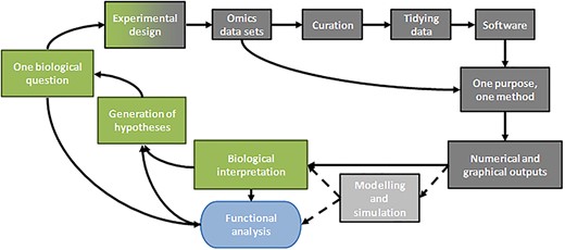
Workflow for our multi-omics integrative studies. The different parts of this article are represented by grey boxes and the green boxes stand for biological concepts that close the workflow. The workflow converges towards the functional analysis required to validate the whole study (blue box). The dotted lines and the light grey box represent another way to use the numerical outputs, not described in this article.
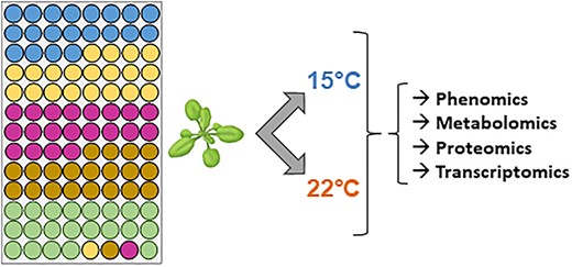
Schematic overview of the strategy and experimental protocol used in this study. Each circle represents one plant and each colour stands for one ecotype of A. thaliana. For each biological replicate grown at 15°C or 22°C, the position of a given ecotype has been changed randomly to avoid position effects. Four free positions in the rack have been completed with one extra plant per ecotype.
Biological context
As a direct consequence of global warming, we have seen alterations in seasons accompanied by a net change in temperature. Among the different possible effects of global warming, temperature increase has been the most studied since this effect has already been clearly observed [20]. Moreover, cold stress can also occur without any prior chilling period, in which case it could become problematic to maintain agricultural productivity in the future [21]. The model plant Arabidopsis thaliana has a worldwide geographical distribution and has therefore had to adapt to multiple and contrasting environmental conditions [22]. The huge accumulation of molecular data concerning this plant is thus very helpful to study complex multiple level responses. It is nevertheless expected that the obtained results can be transferred to other plant species of economic interest [23].
Experimental design
First of all, in deciding the ideal number of biological replicates, a compromise needs to be made; it is often difficult to find an agreement between the reality of the biological experiment (e.g. limitation in material, space, time, work force and cost) and the necessity to get robust information needed for statistical analyses. The method used for randomization of replicates also needs to be considered. For these reasons, the experimental protocol must be tailored to minimize potential external impacts within and between the replicates and avoid confounding effects.
Our experimental design was built using two crossed factors: (i) ecotypes with five levels (four ecotypes, Roch, Grip, Hern and Hosp, growing at different altitudes in the Pyrénées [24] and Col, a reference ecotype from Poland, growing at low altitudes) and (ii) two growth temperatures (22°C and 15°C). Data from rosettes were collected and analysed for each ecotype. Rosettes were collected at the time of floral emergence, i.e. after 4 weeks at 22°C and after 6 weeks at 15°C. More details on the plant culture conditions can be found in a previous publication [18]. Three independent biological replicates were analysed for the five ecotypes cultivated at the two temperatures with 20 plants per ecotype per biological replicate. To minimize the influence of experimental conditions, each plant was grown at a randomly chosen place as per the experimental design represented in Figure 2.
Omics datasets
In this project, the following four omics datasets (called blocks hereafter) were collected:
(i) Phenomics, a macro phenotyping analysis, was performed on rosettes as described previously [18]. Five phenotypic variables were measured: mass, diameter, number of leaves, density, and projected rosette area.
(ii) Metabolomics, which involves the identification and quantification of the seven cell wall monosaccharides (fucose, rhamnose, arabinose, galactose, glucose, xylose and galacturonic acid), was performed using high-performance anion exchange chromatography with pulsed amperometric detection (HPAEC-PAD) [6]. The theoretical cell wall polysaccharide composition was inferred based on monosaccharide analyses [6, 18, 25].
(iii) Proteomics, i.e. the identification and quantification of cell wall proteins, was performed using LC-MS/MS analysis as described in Ref. [6]. Altogether, 364 cell wall proteins (CWPs) were identified and quantified [19].
(iv) Transcriptomics, i.e. the sequencing of transcripts, also known as RNA-seq, was performed according to the standard Illumina protocols described in a previous work [6]. Altogether, 19 763 transcripts were obtained among which the transcripts encoding the 364 CWPs were sorted [19]. These data will be referred to as cell wall transcriptomics dataset hereafter.
Data preprocessing
Statistical data analysis requires efficient data preprocessing: ‘It is often said that 80% of data analysis is spent on the process of cleaning and preparing the data’ [26].
When dealing with biological data from high-throughput technologies, it is necessary to first perform specific preprocessing, such as data filtering, transformation and normalization. These preprocessing steps are fully detailed in two previous works [18, 19].
From a practical point of view, in an integrative analysis framework, each dataset needs to be structured in the same way with biological samples in rows and variables in columns.
Furthermore, handling missing data is always challenging. As stated by the American statistician Gertrude Mary Cox, ‘the best thing to do with missing values is not to have any’. In the same vein and more recently [27], it was also stated that ‘there is NO good way to deal with missing data’ and ‘before jumping to methods of data imputation, we have to understand the reason why data goes missing’. In view of these observations, we developed our own strategy to deal with the missing values in the quantitative proteomics dataset depending on the reasons why such data were missing. Two situations were considered: (i) non-validated proteins (identification with a single specific peptide and/or in a single biological replicate) and (ii) undetectable proteins (no peptide identified under a given condition). In the former case, background noise corresponding to the mean of the minimum and the first statistical quartile of the biological replicate was applied, and for the latter, a background noise of 6 (value lower than the minimum value found in the whole experiment) was applied. Consistent with our framework based on cycles, the choice of strategy was the result of several trials using various methods followed by evaluating how they influenced the results of a principal component analysis (PCA) used as quality control. For instance, replacing missing values with zeros or another unique small value can produce artefacts on both individual and variable representation (e.g. samples isolated or artificially clustered).
Another aspect of missing data is missing rows. This happens if, for instance, the number of biological replicates is not the same in transcriptomics and proteomics analyses. In our case, two out of the 30 replicates of the transcriptomics data had to be deleted due to their low quality. Following the method proposed in Ref. [28], these missing rows were imputed using the samples for which all the data were available, i.e. the two other replicates.
Rationale supporting the proposed framework
Software
As mentioned in the Comprehensive R Archive Network (CRAN, cran.r-project.org), R ‘is a freely available language and environment for statistical computing and graphics which provides a wide variety of statistical and graphical techniques...’. R functions with a command-line interface that allows to build scripts that can be run on various datasets with little tuning. R also gives free access to the latest developments in methodology, thanks to its very active community of users committed to providing open access in the spirit of open science. In addition, efficient tools such as RStudio (www.rstudio.com) have been developed to facilitate initiation to R. Furthermore, many resources are available on CRAN to learn R, and the Bioconductor repository (www.bioconductor.org) provides tools for the analysis of high-throughput genomic data [29].
There exist several R packages that address statistical integrative studies. We focus on the mixOmics package [16, 30], but other packages, such as FactoMineR [31], can also be used. Also viable are methodologies developed to study a mixture of quantitative, categorical and frequency data [32] and for multiway discriminant analysis [33], as well as the Multi-Omics Factor Analysis approach [34]. With respect to commercial software, SIMCA-P (Umetrics, umetrics.com) proposes several methods to perform integrative analyses, and toolboxes for Matlab are available (The MathWorks, Inc., Natick, MA, USA). We preferred to use an open-source software, which provides easier access for nonspecialists than a commercial one [35]. Furthermore, mixOmics appears to be a very active package addressing data integration issues and has been downloaded more than 20 000 times in 2019 from the Bioconductor repository, and the corresponding reference [30] has been cited more than 300 times to date.
One purpose, one method
In this section, in part inspired by the mixOmics tutorial (mixomics.org/methods), we highlight the link between a biological question and the appropriate statistical method that is used to describe it. These methods are either unsupervised or supervised depending on the biological question to be answered. It is crucial to distinguish the two cases to correctly interpret the results:
(i) Purpose: To explore one single quantitative variable (e.g. the level of expression of one gene). Method: univariate elementary statistics such as mean, median for the main trends and standard deviation or variance for dispersion, which can be further complemented with a graphical representation such as boxplot.
(ii) Purpose: To assess the influence of one single categorical variable on a quantitative variable (e.g. is the plant growth different in two or more environmental conditions?). Method: Statistical significance test, such as the Student’s t-test or Wilcoxon rank sum test for the two groups and ANOVA or Kruskall–Wallis for cases with more than two groups [36]. These methods have sometimes to be adapted to take into account the specificity of some datasets (count, continuous or compositional data). Furthermore, the multiplicity in statistical testing when handling many variables has to be controlled using methods such as Benjamini–Hochberg (false discovery rate control) or Bonferroni. Special attention must be paid to the structure of the data: independent samples (e.g. independent groups observed under various conditions) or paired samples (e.g. the same sample observed twice or more under various conditions).
(iii) Purpose: To evaluate the relationships between two quantitative variables (e.g. is there a correlation between the amount of a given protein and the related transcript abundance?). Method: correlation coefficients (Pearson for linear relationships and Spearman for monotonous ones) [36]. Graphical representations of correlation matrices can provide a global overview of pairwise indicators [37, 38].
(iv) Purpose: To explore a single dataset (e.g. transcriptomics) and identify the trends or patterns in the data, experimental bias, or identify if the samples ‘naturally’ cluster according to the biological conditions (e.g. can we observe the effect of different environmental growth conditions on different ecotypes?). Method: Unsupervised factorial analysis such as PCA [39] provides such information about one dataset without any a priori. When dealing with omics data, centring and scaling the data so that all variables have zero mean and unit variance prior to performing PCA is usually useful to obtain meaningful PCA results.
The above-mentioned methods are standard and routinely used for biological data analysis, while the methods mentioned hereafter are less common:
(i) Purpose: To classify samples into known classes based on a single dataset (e.g. can we classify various ecotypes according to their transcriptomics profiles?). Method: Supervised classification methods such as partial least squares (or projection to latent structures) discriminant analysis (PLS-DA) [40] can be used to assess how informative the data are to correctly classify the samples, as well as to predict the class of new samples.
(ii) Purpose: To unravel the information contained in two datasets, where two types of variables are measured on the same sample (e.g. can we identify groups of proteins varying in the same way or in an opposite way as groups of transcripts?). Method: Using partial least squares (or projection to latent structures, PLS)-related methods [41] allows to determine if common information can be extracted from the two datasets (or elucidate the relationship between them).
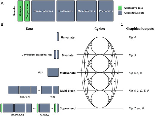
One purpose, one method concept to analyse qualitative and quantitative blocks. (A) Schematic representation of the different blocks (or datasets) co-analysed in this study. The samples are represented in rows and the variables in columns. (B) Schematic overview of the methods implemented. Methods are represented in the form of cycles within an integrated study. (C) Examples of graphical outputs detailed in the Results section. Qualitative and quantitative blocks are represented in green and grey, respectively. DA, discriminant analysis; MB, multi-blocks; PCA, principal component analysis; PLS, partial least squares.
The following multi-table methods are very recent, and there are relatively few applications that have been published so far for these methods. We expect that present work will contribute to increasing the application of these methods for biological datasets:
(i) Purpose: The same as the previous goal but taking more than two datasets into consideration (e.g. what are the main relationships between the proteomics, transcriptomics and phenotypic data?). Method: multi-block PLS-related methods.
(ii) Purpose: The same as the previous objective but in a supervised context (e.g. can we determine a multi-omics signature to classify ecotypes?). Method: Multi-block PLS-DA (referred as DIABLO for Data Integration Analysis for Biomarker discovery using Latent variable approaches for Omics studies) [10].
A schematic view of the datasets considered and the methods used in this study is presented in Figure 3. The different steps in an integrative statistical study are illustrated through several cycles (Figure 3B). We prefer this scheme rather than one in the form of a straight pipeline beginning with univariate analysis and ending with multi-block approaches. Each of these methods contributes to the global comprehension of the data and can agree with or contradict others. Univariate statistics may highlight outliers or essential variables, and multi-block approaches may draw attention to samples and/or variables showing specific behaviour that should be studied through a univariate method. We believe that for any statistical analysis to be relevant, it must go through these cycles with progress and feedback.
Sparse extensions
All the methods developed in mixOmics are associated with a sparse extension [sparse PCA (S-PCA), sparse PLS (S-PLS) to name a few]. Sparse methods are useful to remove variables that are noninformative with respect to the purpose of the multivariate method. Sparse PCA only selects those variables that contribute highly to the definition of each principal component (PC) and removes others. Sparsity is mathematically achieved via least absolute shrinkage and selection operator (LASSO) penalizations [42].
In the context of omics data (where the number of variables is much larger than the number of observations), using sparse methods is very practical as it reduces the number of potentially relevant variables displayed on the graphical outputs thereby facilitating the biological interpretation of results and also minimizing the list of potential candidates for further investigations. The number of variables to be selected highly depends on what will be done subsequently. The user can therefore ask for a selection of a limited number of variables in cases where the biological validation necessitates a new laboratory experiment. On the contrary, hundreds of variables can be selected if the list of candidates is submitted to databases to evaluate biological functions or metabolic pathways enriched in the list. The mixOmics package provides functions (tune.splsda, for instance, as illustrated in the script provided as Supplementary Material in a dedicated section titled ‘Tuning the number of selected variables’) that implement a cross-validation strategy to evaluate the optimal number of variables to be selected for each component. Consistent with our framework consisting of cycles, several trials have to be run varying the number of selected variables and evaluating the results both from statistical and biological points of view. For instance, we suggest running the sparse methods with parts of the data varying from 75, 50, 25, 10, 5 to 1%. The statistical point of view is provided by the cross-validation framework in tune functions previously mentioned. The biological point of view relies on the relevance and interpretability of the results. A good trade-off between both points of view consists in choosing a number of variables with a good cross-validation criterion (even if not the better) and providing meaningful results. When working with omics datasets, the number of variables to select can be higher than 1000. If functional analyses have to be performed, it cannot apply to so many candidates.
Furthermore, as LASSO is known to produce unstable results, we decided to focus on those variables, which are the most frequently selected in a cross-validation strategy. We illustrate this point in the Supplementary Material section showing the results of the perf function.
Numerical and graphical outputs
The results obtained for the univariate and bivariate approaches are reported mainly as P-values for statistical testing. Boxplots and bar plots, produced, for instance, by the ggplot2 package [43], may help in the interpretation of results (Figure 3C). We also used graphical representations of correlation matrices (Figure 3C) such as those produced by the corrplot package [44]. This is essential even when dealing with a relatively low number of variables; for example, with only 50 variables, 1225 (50 × 49/2) pairwise correlation coefficients are computed that need to be analysed and interpreted.
Regarding multivariate analyses (from PCA to multi-block analyses), we used the graphical outputs provided by the mixOmics R package [16]. These are based on the representation of individuals and variables projected on specific sub-spaces (Figure 3C). A thorough discussion on the complementarity between several graphical displays is given in a previous work [17]. In a multivariate supervised analysis, the individuals (biological samples) of a study are represented as points located in a specific sub-space defined by the first components (Figure 3C), and data interpretation is based on the relative proximities of the samples and on the equivalent representation for variables.
The standard representation for variable plots is frequently referred to as the correlation circle plot (Figure 3C). This plot was primarily used for PCA to visualize relationships between variables but has been extended to deal with multi-block analysis. In such a plot, the correlation between two variables can be visualized through the cosine of the angle between two vectors starting at the origin and ending at the location of the point representing the variable. The representation of variables can also be done through a relevance network [45, 46]. In our specific context, these networks are inferred using a pairwise similarity score analogous but not identical to a Pearson correlation coefficient and directly obtained from the outputs of integrative approaches [17]. A Circos plot [10] can be traced to represent relationships between and within selected variables from each dataset in a multi-block analysis. Based on the same pairwise similarity matrix used for a relevance network, a clustered image map can then be displayed. This type of representation is based on hierarchical clustering simultaneously operating on the rows and columns of a real-valued similarity matrix. This is graphically represented as a two-dimensional coloured image, where each entry of the matrix is coloured on the basis of its value while the rows and columns are reordered according to hierarchical clustering.
Results
In this section, we have provided neither a thorough biological interpretation of the results nor a comprehensive description of every statistical analysis performed. Instead, we highlight the limits of each method that lead to the next step of the statistical analysis and show how a biologist can interpret and make use of the conclusions from a statistical study.
Univariate and bivariate analyses
We illustrate univariate analysis through graphical representations of phenotypic data linked to a single parameter of the experimental design. Figure 4A displays parallel boxplots as well as individual observations of the number of leaves for the five ecotypes grown at two temperature conditions. Figure 4B only displays average values from three measurements for each ecotype and temperature.
![Examples of graphical outputs of a supervised bivariate analysis illustrated by (A) boxplot (each colour corresponds to the different values obtained for each triplicate) and (B) individual plot (each colour corresponds to the average obtained for one triplicate, and does not match with that used in (A). Five A. thaliana ecotypes (Col, Roch, Grip, Hern and Hosp) and two growth temperatures (22°C and 15°C) were used. These plots were obtained using functions geom_point() and geom_boxplot() from the ggplot2 package [43].](https://oup.silverchair-cdn.com/oup/backfile/Content_public/Journal/bib/22/3/10.1093_bib_bbaa166/1/m_bbaa166f4.jpeg?Expires=1749223649&Signature=4D1NTPUhexgzAvQ3v-Vb2EQJrAWH9glq3exwmwBYHb~93Xf8Aj7TqDPzXBuaJ9oUw1BGKfU3lmDe67Ej8WcQD-h2YHohxF4ZnRWtUAz8D~uJcF6Ow1NFoJlL0QfWXC871CeT~~u387MyRUv9meHmrne9Bd6tHa4Xy~4KxA7j-rARMn3wCjr1ICgy~XZ3wJrNoj8hZEDhaiZ4bxf257-TBT4cXiq4l-f69XWUqxSNiEMu7CuRD18Cv1Ks5UgasWxGWn~dl2pIwD5WSEr1KXoQwkpjNsSarpZxvzq7Ox1JuAoabyiAZdaMq0wosdrtVk9IU3BdbJeSqq55m268W98mFQ__&Key-Pair-Id=APKAIE5G5CRDK6RD3PGA)
Examples of graphical outputs of a supervised bivariate analysis illustrated by (A) boxplot (each colour corresponds to the different values obtained for each triplicate) and (B) individual plot (each colour corresponds to the average obtained for one triplicate, and does not match with that used in (A). Five A. thaliana ecotypes (Col, Roch, Grip, Hern and Hosp) and two growth temperatures (22°C and 15°C) were used. These plots were obtained using functions geom_point() and geom_boxplot() from the ggplot2 package [43].
The quality of data is evident from the graphics. The relatively low scattering of points representing individuals of each biological replicate (Figure 4A) indicates the rather good reproducibility between the samples and the biological replicates, which means that values from several plants of a given biological replicate can be averaged in the subsequent steps. The trend observed visually in Figure 4B regarding the temperature and ecotype effects can be confirmed via statistical testing, such as two-way ANOVA [47] (results not shown). However, this analysis does not give any information about how the variables interact with each other. This lack of complexity in the analysis has compelled us to use other methods when dealing with the entire dataset as described below.
The bivariate analysis is illustrated on the rosettes cell wall transcriptomics dataset composed of 364 variables (or transcripts). The first way to explore the whole dataset can be through computing pairwise correlation coefficients. For instance, Figure 5 displays the correlation matrix between samples and indicates that the levels of transcript accumulation for each sample are positively correlated with all the others.
![Graphical representation of multivariate analysis showing pairwise correlation coefficients of cell wall transcriptomics datasets of the five A. thaliana ecotypes grown at 15°C or 22°C. The colour code and the ellipse size represent the correlation coefficient between the levels of transcript accumulation for each sample. Both the area and the eccentricity of the ellipse represent the absolute value of the corresponding correlation coefficient; the orientation of the ellipse determines the sign of the corresponding correlation coefficient. This plot was obtained using the function corrplot() from the corrplot package [44].](https://oup.silverchair-cdn.com/oup/backfile/Content_public/Journal/bib/22/3/10.1093_bib_bbaa166/1/m_bbaa166f5.jpeg?Expires=1749223649&Signature=J7BI6iPq8EG0S43p5x2YE4HIDVnCRjBJIPR-gasGSRJ-uu9rWLAOqgJdRfpGI7IShaJioeadbd6S1113rvUMvLUIVAZ31MyexYA9ujubkLzWtA0xPuRxr0uXNA0DPJLQO9MbM6yWpaDiTfd0n9qTLwfG8xPEd7pO3nhCp2hgfMXU0RHEDRkd7mTsUjs5OYzlxGj69Azj~TbI6J-MBrR1o~YLlne~t6vvZ0tCG7jNGg5ezb6HZ2TQFnSr7fP20iYkZ6ki6nj1p9RiwCrE62Xwsr8pUg35qqOejfhznqB4EBKDY5dHzTKMmw9gxK2xu9yEC38zL9NsuO58KOxa1DGFfQ__&Key-Pair-Id=APKAIE5G5CRDK6RD3PGA)
Graphical representation of multivariate analysis showing pairwise correlation coefficients of cell wall transcriptomics datasets of the five A. thaliana ecotypes grown at 15°C or 22°C. The colour code and the ellipse size represent the correlation coefficient between the levels of transcript accumulation for each sample. Both the area and the eccentricity of the ellipse represent the absolute value of the corresponding correlation coefficient; the orientation of the ellipse determines the sign of the corresponding correlation coefficient. This plot was obtained using the function corrplot() from the corrplot package [44].
Multivariate analysis
A PCA can then be performed as an extension of quality control as mentioned before. Figure 6A highlights the distance between the three replicates from one condition. We observe that the Grip ecotype is well clustered, whereas the Col ecotype is more scattered. However, it is reminded that due to the rather low proportion of variance exhibited by the first two PCs displayed here, the absoluteness of the results have to be taken with caution, considering the following components could be meaningful to consolidate and confirm our results.
![Graphical representation of unsupervised (A, B) and supervised (C–F) analyses of the rosette cell wall transcriptomes of ecotypes grown at 22°C or 15°C. (A) Individuals plot of a PCA from ecotypes grown at 22°C (dark colours) and 15°C (light colours) associated with (B) variable plot. (C) Individual plot of a PLS-DA from ecotypes grown at 22°C (orange) and 15°C (blue) associated with (D) variable plot and (E) individual plot of a S-PLS-DA associated with (F) variable plot. Two circles of radius 1 and 0.5 are plotted in each variables plot to reveal the correlation structure of the variables. These plots were obtained using the functions pca(), plsda(), plotIndiv() and plotVar() from the mixOmics package [16].](https://oup.silverchair-cdn.com/oup/backfile/Content_public/Journal/bib/22/3/10.1093_bib_bbaa166/1/m_bbaa166f6.jpeg?Expires=1749223649&Signature=i-YlP1LVAF2YtOSEGK83R71YKL~SohhMXWgEU67RCn~zzrHa9WvkH3lV7IWy2O7XRC84KQVhwNQHQIsaLZR2WbYqmYrgQqeB9ky9djaoGw4gbUQmUHXPzS4p~WkM4QZS09Y-4cuBO4H8jxHGsewwjxx~JDgRsFLTpadrTg3uVLcsuo1PiHthpUO-wDHHTXAaCc0uwMxvWt7HxE0rYJkY1RHRPhjknJlfA7HRDoJBS2SsyCNM7YciXXFHfQV0TwRE1wCieNrIeNGwmALyJTUCVqglZMRJsJO94HZ-cQZ1KnKO4pZ9mb8uoF~yLdzKbiLnOVhfPIdT4mpP7V4bQ0lQ~Q__&Key-Pair-Id=APKAIE5G5CRDK6RD3PGA)
Graphical representation of unsupervised (A, B) and supervised (C–F) analyses of the rosette cell wall transcriptomes of ecotypes grown at 22°C or 15°C. (A) Individuals plot of a PCA from ecotypes grown at 22°C (dark colours) and 15°C (light colours) associated with (B) variable plot. (C) Individual plot of a PLS-DA from ecotypes grown at 22°C (orange) and 15°C (blue) associated with (D) variable plot and (E) individual plot of a S-PLS-DA associated with (F) variable plot. Two circles of radius 1 and 0.5 are plotted in each variables plot to reveal the correlation structure of the variables. These plots were obtained using the functions pca(), plsda(), plotIndiv() and plotVar() from the mixOmics package [16].
However, the interpretation of the PCA shows us a first trend. Indeed, the samples are clearly separated along the first (horizontal) axis according to temperature: samples grown at 22°C are all located on the left (negative coordinates on PC1), whereas samples cultivated at 15°C are on the right. This indicates that the effect of temperature is stronger than that of ecotypes because PC1 captures the most important source of variability in the data. The representation of variables, i.e. the transcripts (Figure 6B), is not of great interest at this step; it mainly highlights the need for selection methods to facilitate the interpretation of results in terms of gene expression level. However, interpreting such a plot jointly with the individual plot enables, for instance, to identify overexpressed genes in samples grown at 15°C, which are located on the right side on the variables plot, as well as in the individual plot (Figure 6A).
Supervised analysis and variable selection
To illustrate a supervised analysis, we used the same dataset as before (cell wall transcriptomics for the quantitative block) to discriminate the samples according to temperature (qualitative block) by performing a PLS-DA analysis. A similar analysis could be carried out with the ecotypes, but the interpretation of results would be more complicated with five categories instead of two. Moreover, we have already seen that the temperature effect is the strongest for this dataset (Figure 6A). To enhance interpretability of the results, we now consider the sparse version of PLS-DA to select the most discriminant genes for the temperature effect. After several trials, we decided to select 20 genes on each component as a good trade-off between the results of tune.splsda and the interpretability of the graphics as stated in Sparse extensions section.
Figure 6 also displays the results of PLS-DA (C, D) and sparse PLS-DA (S-PLS-DA) (E, F). Individual plots (Figure 6C and E) and variable plots (Figure 6D and F) are interpreted in the same way as PCAs. Individual plots only use two colours corresponding to the two temperatures. In both cases, the discrimination between the samples is clear-cut (Figure 6C and E). This result confirms the overriding effect of the growth temperature. The result of S-PLS-DA indicates that discrimination can be observed with only a few genes. The most relevant genes displayed in Figure 6F have to be validated through functional analysis, but these developments are outside the scope of this article.
This example highlights the specificity of a supervised analysis: it allows studying the impact of the different experimental parameters (in this case, the temperature) on the quantitative variables. Thus, results obtained from this analysis, in addition to enabling biologists to find answers to questions concerning the biological system under study, could lead to prospective applications in many areas.
Multi-block analyses
Multi-block analyses can address the main purpose of an integrative study by analysing together all the blocks acquired for each sample. As an illustration, we expose the results of a five-block supervised analysis considering phenotypic, cell wall transcriptomics, proteomics and metabolomics as quantitative variables and temperature as the categorical block.
![Graphical representation of a multi-block analysis performed on the rosettes of ecotypes grown at 22°C (orange) or 15°C (blue). (A) plotDIABLO showing the correlation between components from each dataset maximized as specified in the design matrix. (B) Individual plot projects each sample into the space spanned by the components of each block associated with (C) variable plot highlighting the contribution of each selected variable to each component. (D) Clustered image map of the variables (protein, red; transcripts, green; metabolites, grey; phenotypes, black) to represent the multi-omics profiles for each sample (15°C: blue, 22°C: orange). These plots were obtained using the functions block.splsda(), plotIndiv(), plotVar() and cim() from the mixOmics package [16].](https://oup.silverchair-cdn.com/oup/backfile/Content_public/Journal/bib/22/3/10.1093_bib_bbaa166/1/m_bbaa166f7.jpeg?Expires=1749223649&Signature=YhUH1g4u3YdbrQMmQsnOkA919syg9a8SgkrDMRD2LVtnnI0nxsXQuBK3mjsH4fxvHGPlD~oqfBdZuci9h3KuS1r8l6IdvFlOEvZvpxu9EGKoq6rqFgFKPlTjmTPIoCfValENDl2rkck115X0onz1rNGDcJNcHbRE-kpKixIQ2CcuQAqK5fRbsOL3nL0wYpNddkQAMUrEJVDHuLQ6bM1VomIpCrFf9fIPutUnNU5Wq~R1M0NjVE-VdXTV4ZTV8yuPnOjvW06y~1KuNrk9MclIo8jDmBg5j4qKwVZ27mUWgzXV~m73wQnj6w1brVJ-Cfx0QlY95hquqCgCfPP2SYQG7Q__&Key-Pair-Id=APKAIE5G5CRDK6RD3PGA)
Graphical representation of a multi-block analysis performed on the rosettes of ecotypes grown at 22°C (orange) or 15°C (blue). (A) plotDIABLO showing the correlation between components from each dataset maximized as specified in the design matrix. (B) Individual plot projects each sample into the space spanned by the components of each block associated with (C) variable plot highlighting the contribution of each selected variable to each component. (D) Clustered image map of the variables (protein, red; transcripts, green; metabolites, grey; phenotypes, black) to represent the multi-omics profiles for each sample (15°C: blue, 22°C: orange). These plots were obtained using the functions block.splsda(), plotIndiv(), plotVar() and cim() from the mixOmics package [16].
The statistical relationships between blocks must be defined by the user through a design matrix. This is a square matrix with as many rows and columns as the number of blocks. It is symmetric and contains values between 0 and 1. A value close to or equal to 1 indicates a strong positive relationship between the blocks to be integrated, and a value close to 0 indicates weak or no relationship. Fixing the values in the design matrix is complex. To simplify, the values of 0 and 1 can be used from a binary point of view: either blocks are linked, or they are not. In a supervised context, the values also help to achieve a balance between optimizing relationships between quantitative blocks and the discrimination of outcome. As stated in [10], the design matrix can be determined using either prior biological knowledge or a data-driven approach. The latter is consistent with our framework as it uses the results of pairwise analyses with PLS methods to decide to link two blocks in the design matrix. In our example, for illustration purpose, we considered a design matrix composed of 0 between blocks to favour the task of discrimination rather than the relationships between the blocks.
The interpretation of a multi-block supervised analysis requires several graphical outputs. Some of them are presented in Figure 7 for the sparse version. The result of the multi-block supervised analysis without selection is presented in Supplementary Material available online at https://dbpia.nl.go.kr/bib. Figure 7A represents the correlation between the first components from each dataset. Such a plot also allows assessing the influence of the design matrix [11]. In Supplementary Material available online at https://dbpia.nl.go.kr/bib, we present results of multi-block analysis using three design matrices as described in [16]: null as we used for illustration purpose, full (replacing 0 with 1) to emphasize the relationships between blocks and full-weighted (replacing 0 with 0.1) to lower the influence of the relationships between blocks. In our example, the design matrix is not so important, but we recommend trying at least three design matrices corresponding to the null, full and full-weighted as previously mentioned.
![Example of network representation. (A) A Circos plot representing the correlations between variables within and between each block (edges inside the circle) and showing the average value of each variable in each condition (line profile outside the circle). (B) Network displaying the correlation between the cell wall transcriptomics (.T, green) and the proteomics data (.P, red) in accordance with the colour code. These plots were obtained using the functions circosPlot() and network() from the package mixOmics [16].](https://oup.silverchair-cdn.com/oup/backfile/Content_public/Journal/bib/22/3/10.1093_bib_bbaa166/1/m_bbaa166f8.jpeg?Expires=1749223649&Signature=RAeVRTQj1MzX154b2yAmynPsIVas5nmXeiyZIuPYcqO14lHetdGf33~Wb1rF-L66qQtaxjNPJ7uDJASRlqd8rOGfg2vDKaOCQbmq4KOIZRepwJwKiahQGU3FCo5cZuym--8ciX8OvO5vCyb~UrpUjwDXcJWcFBEu9gjIUgYgV2ZZMvwRoozyrex0t9WjNxFQZV20e7NxQWKX8XacmIXjgU2fiEyKtH8ImpaeKCeX2f-3v9AZi6LhtkUmtLmsxRmunwySrermE-ITs1qpKXUmd7p-2Sa8YIlZz3bY-02YYEvWPyCjzZ~ROlZmxU48~~go-AylvIs7uYaFHQeZYNFuTg__&Key-Pair-Id=APKAIE5G5CRDK6RD3PGA)
Example of network representation. (A) A Circos plot representing the correlations between variables within and between each block (edges inside the circle) and showing the average value of each variable in each condition (line profile outside the circle). (B) Network displaying the correlation between the cell wall transcriptomics (.T, green) and the proteomics data (.P, red) in accordance with the colour code. These plots were obtained using the functions circosPlot() and network() from the package mixOmics [16].
Globally, the correlation values in Figure 7A are close to 1, and this is mainly due to the separation of the two categories (22°C versus 15°C) through a design matrix thus favouring the discrimination task. With a full design matrix, we get higher correlation values but less separated groups. Regarding the individual plots (Figure 7B), it appears that discrimination is better for the cell wall transcriptomics and proteomics blocks than for the others. The samples plot (Figure 7B) also has to be interpreted together with the variables plot (Figure 7C). Using the results of the sparse version of the multi-block analysis, we can easily identify variables from each block that are mainly involved in discrimination according to the growth temperature. For instance, variables located on the right on the correlation circle plot (Figure 7C) contribute to discrimination between the samples grown at 22°C because these are also located on the right in the individual plots (Figure 7B). Another way to display the results is presented in Figure 7D. The clustered image map highlights the profiles of selected variables among the samples. It also includes the results of hierarchical clustering performed jointly on variables and samples. Regarding samples, the two groups based on temperature are visualized with the help of the dendrogram on the left. Note however, that cluster gathering samples at 15°C can be divided into two subclusters with the Col ecotype in its own subcluster. Regarding variables, the graphic mainly points out global trends in the behaviour of selected variables. The interpretation can then lead to retro analyses to validate candidates. This can be done through new statistical analyses as well as new biological experiments [48].
Relevance networks
Another way to interpret the results of a multi-block approach consists in producing a Circos plot. On Figure 8A, the variables are sorted first according to their block and then depending on their importance in discrimination. An edge links two nodes if their correlation is higher than a threshold which is subjectively set by the user. We recommend experimenting with different thresholds varying from 1 to 0 by 0.1, to explore several configurations of this rather complex graphical display. The resulting networks will display more and more edges. For instance, a relevant threshold can be determined slightly above a value that involves an abrupt increasing in the number of edges. In Figure 8A, we chose 0.9 for the purpose of illustration as it appears to provide reasonable readability.
The relationships are mainly positive and concern a few variables from each block. To complete the interpretation, we focus on another network generated with only two blocks (Figure 8B, cell wall transcriptomics and proteomics), which accentuates the relationships between pairs of proteins and transcripts. The selection of variables is a valuable information for the biologist in that it allows to focus on this smaller selection for validation and draw biological conclusions from it.
Relevance networks can also be viewed as an initial step in modelling since they mimic biological networks and provide clues to address inference networks issues through further dedicated experiments.
Conclusion
In the context of integrative biology, a very large volume of data is produced, which can be heterogeneous and need adapted and specific statistical methods for their interpretation. Even if multi-block approaches can be viewed as the best tools to address a given issue, other more basic standard statistical methods (univariate for instance) must not be overlooked. A deep understanding of a biological phenomenon requires a sequence of various approaches to analyse the data. The statistical analysis of large omics datasets can be extremely time-consuming because each step of the framework provides information. An approach alternating the use of different statistical methods combined with a critical interpretation of results helps to progress towards a consistent assumption for an in-depth experimental validation. The results presented in this case study could not have been obtained using standard statistical approaches.
We propose a powerful framework to manage and analyse multi-omics heterogeneous data to carry out an integrative statistical analysis.
We illustrate this framework through a study to investigate the cell wall plasticity of plants exposed to sub-optimal temperature growth conditions.
We highlight the fact that each statistical method used in this framework addresses a specific biological issue.
Our framework illustrates a pathway that extends from basic univariate statistics to the most recent methodologies in multi-block integration analysis.
Acknowledgements
The authors thank Dr Kim-Anh Lê Cao, Dr Philippe Besse and François Bartolo for their support and help with graphical outputs and interpretation of multi-block analysis.
Funding
The authors thank Toulouse University III-Paul Sabatier and the Centre National de la Recherche Scientifique (CNRS) for financial support. H.D. acknowledges financial support from Midi-Pyrénées Region and the Federal University of Toulouse (IDEX UNITI (2015-230-CIF-D-DRD IDEX UNITI WALLOMICS). French Laboratory of Excellence project ‘TULIP’ (ANR-10-LABX-41; ANR-11-IDEX-0002-02).
Harold Duruflé is a postdoctoral researcher at INRAE. He develops a system biology approach consisting of a vertical integration of different levels of information to highlight molecular interactions in complex biological processes.
Merwann Selmani contributed to this work during an internship as an undergraduate student at the Laboratoire de Recherche en Sciences Végétales and the Institut de Mathématiques de Toulouse.
Philippe Ranocha is a researcher at CNRS, France. He works mainly on the functional study of multigenic families related to ROS homeostasis.
Elisabeth Jamet is a research director at CNRS and studies plant cell walls. She has developed integrative approaches to treat omics data and identify genes involved in cell wall plasticity under environmental constraints.
Christophe Dunand is a professor at Toulouse University III-Paul Sabatier. His main interest is in integrated approaches to study the evolution of multigenic families related to ROS homeostasis and their function in response to environmental changes.
Sébastien Déjean is a research engineer at the Institut de Mathématiques, Toulouse University, and works on interdisciplinary research projects involving statistical analyses of complex and heterogeneous datasets.
