


Abstract
Accurately predicting protein–ligand binding affinities can substantially facilitate the drug discovery process, but it remains as a difficult problem. To tackle the challenge, many computational methods have been proposed. Among these methods, free energy-based simulations and machine learning-based scoring functions can potentially provide accurate predictions. In this paper, we review these two classes of methods, following a number of thermodynamic cycles for the free energy-based simulations and a feature-representation taxonomy for the machine learning-based scoring functions. More recent deep learning-based predictions, where a hierarchy of feature representations are generally extracted, are also reviewed. Strengths and weaknesses of the two classes of methods, coupled with future directions for improvements, are comparatively discussed.
Introduction
Molecular recognition is of central importance to many biological functions and systems, such as enzyme catalysis and intracellular signal transduction. Small-molecule ligands can modulate key intracellular signaling pathways by inhibiting protein functions or triggering protein conformational changes, which makes the identification and design of bioactive molecules a topic of interest. The specificity and strength of a ligand binding to a target protein determines its therapeutic effect, and therefore the accurate prediction of protein–ligand binding affinity plays a crucial role in drug discovery. Owing to the rapid advances in computer power and methodology, computer-aided drug design (CADD) has thrived in the past decade, aiming to vigorously assist the traditional expensive drug trials. An important step in CADD is structure-based virtual screening (VS), whose goal is to computationally test a large pool of ligands and recognize bioactive ligands for further experimental screening. The underlying technique is molecular docking that comprises two major tasks of pose identification and scoring. Current algorithms are capable of identifying ligand poses that are close to the co-crystallized structures (holo structures). However, accurately scoring or predicting the binding affinity remains a challenging problem.
A conjunction of all-atom molecular dynamics (MD) simulation and efficient free-energy sampling algorithms can provide accurate prediction of binding free energies of ligands to proteins, which results in a broad category of prediction methods. By analyzing the simulations, these methods attempt to determine the free-energy difference upon binding or between two similar ligands via a thermodynamic path. Recognized as the most rigorous option for providing free-energy estimates, free energy perturbation (FEP) or thermodynamic integration (TI) considers the relaxation process (by different windows) in the protein/solvent system and applies statistical mechanisms in the calculations [8, 48, 71, 78]. Unfortunately, these methods often struggle in achieving a speed–accuracy balance [91]. Biased MD simulations (umbrella sampling) provide free energies along a reaction coordinate between two thermodynamic states and efficiently sample the whole coordinate by introducing a bias potential to the system [7, 54, 74]. Biased simulations might be preferred over FEP/TI methods due to the integration errors in those methods. However, new free parameters in biased simulations further increase the model complexity [54]. The microscopic all-atom linear response approximation (LRA) and its variants are an alternative method, which approximates the electrostatic free energy by LRA and the nonelectrostatic part by different strategies [90]. Variants, such as the linear interaction energy (LIE) method, attempt to approximate FEP/TI calculations while efficiently reducing the high computational cost [35]. Another broadly used method is the molecular mechanics Poisson–Boltzmann/surface area (MM-PB/SA). In this method, the binding free energy is contributed by the molecular mechanics (MM) energy, the solvation free energy with Poisson–Boltzmann (PB) or generalized Born (GB) calculations, and the entropy terms [58, 87]. Although much faster than FEP/TI methods, MM-PB/SA is challenged by some researchers with its lack of theoretical foundation [84]. These expensive free-energy calculations are considered accurate, but they are often limited to family-specific applications.
Apart from the rigorous but expensive free energy-based simulations, a wide variety of scoring functions for fast predicting protein–ligand binding affinity have been proposed. Although different from free energy-based simulations in accounting for necessary physical processes in molecular recognition, these scoring functions can be applied efficiently to large-scale calculations. Classical scoring functions can be categorized into force field, knowledge-base or empirical [5, 32, 42, 109]. Force field scoring functions measure the binding in a complex by summing up different energy terms that stem from bonded and non-bonded interactions, with the parameters estimated from the experiment data or QM [41]. Entropy contributions are generally neglected in these force fields. Knowledge-based scoring functions are pseudo-energy functions, which arise from a knowledge base comprising the 3D coordinates of a large set of complexes and evaluate the binding in a new complex according to the similarity of its features to those in the knowledge base [31]. A typical knowledge-based potential concerns the ratio of the probability distributions of atom-type pairs spanning a specific distance to a reference distribution and is processed with a reverse Boltzmann method. Empirical scoring functions each stand on an energy factorization model and estimate the binding affinity by a weighted sum of different terms in the model [27, 32, 115]. The weights are calibrated from experiment data, mostly through multivariate regression analysis. It is noteworthy that these classical scoring functions mostly predefine an additive model for different contributors (characterization variables) and thereafter assume a linear relation between such contributors and the predicted binding affinity [5]. However, the assumptions or predefined functional forms may limit their prediction or generalization capability. Without assuming a specific functional form, machine learning-based scoring functions have become an emerging class and burgeoned during the past decade. These functions can implicitly capture different binding contributors arising from any possible kind of interaction, by a linear or nonlinear fit to the experiment data. Still, these scoring functions rely heavily on feature engineering, which uses expert knowledge or statistical inference to define rules for feature representations. In the studies of protein–ligand affinity prediction, such feature representations can vary from simple geometrical and physico-chemical descriptors (e.g. counts of atom pairs, counts of hydrogen bonds, etc.) to more complicated forms (e.g. molecular fingerprints, proteochemometric characterization, etc.). Allowing for simplified feature engineering, deep-learning models learn a hierarchy of feature representations that are relevant for the given task from a simple input representation, leading to a vast number of applications in many research fields. Deep-learning techniques have also been applied to the structure-based studies of protein–ligand binding. These data-driven methods are mostly efficient, while may be questioned about their interpretability or generalization capability.
In this paper, we aim to provide a comprehensive review on the more rigorous free energy-based simulations and the data-driven machine learning-based scoring functions. The wide variety of classical scoring functions, with reviews that can be found elsewhere [32, 42], are not the focus of this work. In what follows, we begin with a description of binding affinity and its experimental measurements. Next, we provide an overview of the free energy-based simulations according to various thermodynamic cycles and introduce a series of featurizers tailored for machine learning-based scoring functions. A discussion section is provided at the end of this review.
Binding affinity and experiment measurements
Protein–ligand binding affinity can also be measured according to quantities like inhibition constant |$K_i$| (dissociation constant of the enzyme-inhibitor complex) or |$IC_{50}$| (concentration of inhibitor required to reduce ligand binding by half). In the absence of competition with the substrate of an enzyme, |$K_i$| is regarded as equal to |$K_d$|. Although |$IC_{50}$| is more easily to be determined, comparisons among different experiments are intractable as the |$IC_{50}$| values depend on the initial amount of ligand available to the protein. In this regard, the binding constants (|$K_d$| and |$K_i$|) are more comprehensive for theoretical studies.
Prediction by free energy-based simulations
FEP and TI
In FEP, |$\{\lambda _i| 0\leq \lambda _i\leq 1, i = 0, \ldots , n\}$| can be a series with equal increments (|$\lambda _{i+1}-\lambda _i=\Delta \lambda $|) or with any pattern of spacing, while non-uniform spacing of |$\lambda $|-points were proposed to be a better choice in some studies [13]. Generally, a compromise between the number of windows (precision) and computational cost is required, and |$50\sim 100$| windows were recommended in [13]. The sampling techniques for selecting |$\lambda _i$| in a particular FEP series include classic modeling methods (e.g. double-wide sampling [51], double-ended sampling [9] and overlap sampling [71]) and modern enhanced-sampling methods (e.g. replica exchange [100], orthogonal space tempering [122], replica exchange with solute tempering (REST) [68] and REST2 [112]). Taking double-ended (DE) sampling as an example, one should perform both the forward perturbation (|$\boldsymbol{A}\rightarrow \boldsymbol{B}$|) and its reverse (|$\boldsymbol{B}\rightarrow \boldsymbol{A}$|), and take |$\Delta G^{DE}_{\boldsymbol{A}\rightarrow \boldsymbol{B}}=\frac{1}{2}(\Delta G_{\boldsymbol{A}\rightarrow \boldsymbol{B}}-\Delta G_{\boldsymbol{B}\rightarrow \boldsymbol{A}})$|. Since TI is confined to small |$\lambda $|-steps, it is advisable to use enough small windows (|$\lambda $|-steps) in a discretized TI [13]. Differently, |$\lambda $| is treated as a dynamic variable in |$\lambda $|-dynamics simulations, which enables a simultaneous evaluation of multiple thermodynamic states in a single simulation [57].
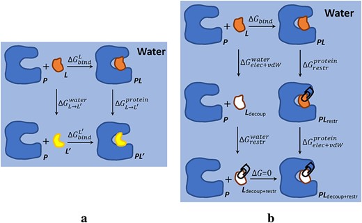
Thermodynamic cycles of calculating protein–ligand binding free energy in FEP methods. (A) Calculating the relative binding free energy of two ligands (|$L$| and |$L^{\prime}$|) binding to a protein (|$P$|) in water. (B) Calculating the absolute binding free energy between a ligand |$L$| and a protein |$P$| in water.
LRA and LIE methods
Thermodynamic cycle of calculating protein–ligand binding free energy in LRA method.
One efficient variant of LRA is the PDLD/S-LRA method [62, 79], which replaces the microscopic potentials |$V_{elec}$| by the effective PDLD/S-LRA potentials |$\bar{V}_{elec}$| [90] in the calculation of electrostatic free energy as |$(\Delta G^{elec}_{bind})^{PDLD/S-LRA}=\frac{1}{2}(\langle \bar{V}_{elec}^{protein}\rangle _{L}+\langle \bar{V}_{elec}^{protein}\rangle _{L^{\prime}}-\langle \bar{V}_{elec}^{water}\rangle _{L}-\langle \bar{V}_{elec}^{water}\rangle _{L^{\prime}})$|. A number of LRA variants involve the estimation of |$\Delta G_{bind}^{^{\prime}}$| by scaled vdW terms (vdW interaction energy between the ligand and its environment), including the LRA/|$\beta $| model with |$(\Delta G_{bind})^{LRA/\beta }=(\Delta G^{elec}_{bind})^{LRA}+\beta (\langle V_{vdW}^{protein}\rangle _{L}-\langle V_{vdW}^{water}\rangle _{L})$| [45] and the PDLD/S-LRA/|$\beta $| model with |$(\Delta G_{bind})^{PDLD/S-LRA/\beta }=(\Delta G^{elec}_{bind})^{PDLD/S-LRA}+\beta (\langle V_{vdW}^{protein}\rangle _{L}-\langle V_{vdW}^{water}\rangle _{L})$| [91]. The LIE method further simplifies the model by neglecting the potentials associated with the non-polar ligand state (|$\langle V_{elec}\rangle _{L^{\prime}}$|) in the calculation of electrostatic free energy [3]. This leads to |$(\Delta G_{bind})^{LIE}=\alpha (\langle V_{elec}^{protein}\rangle _{L}-\langle V_{elec}^{water}\rangle _{L})+\beta (\langle V_{vdW}^{protein}\rangle _{L}-\langle V_{vdW}^{water}\rangle _{L})$|, where |$\alpha $| is a constant around |$\frac{1}{2}$| and |$\beta $| is an empirical parameter [91]. The hydrophobic contribution (e.g. solvent accessible surface area) was additionally considered in [94], yielding |$\Delta G_{bind}=\alpha \Delta G_{bind}^{elec}+\beta \Delta G_{bind}^{vdW}+\gamma \Delta G_{bind}^{hyd}$|. LRA and it variants have been proved to be effective in many protein–ligand affinity predictions [3, 35, 76, 91, 123].
Umbrella sampling methods
During the past few years, umbrella sampling has become a promising approach for determining protein–ligand binding free energies [63, 75, 81]. Normally, the ligand is pulled out of protein active site by an external force (Figure 3), and a series of configurations are generated along the pulling pathway (reaction coordinate) and subjected to umbrella sampling simulations. During the pulling simulation, the protein serves as a reference and the ligand is placed at increasing center-of-mass distance (windows) from the reference with a harmonic bias potential applied to its position. Window-wise simulations based on different starting configurations are conducted with the PMF curves parsed, and a continuous PMF curve over the entire reaction coordinate can be generated by combining the individual PMF curves using WHAM. The absolute binding free energy is then determined as the difference between the peak and valley of this curve [63].
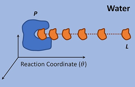
Pulling of a ligand from its protein active site along the reaction coordinate.
MM-PB/SA methods
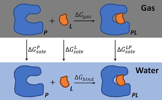
Thermodynamic cycle of MM-PB/SA calculations.
Comparisons in a case study
Modern computer simulations (e.g. MD or MC simulations) reproduce molecular geometry and properties according to MM or QM force fields, which provide the functional form and parameters for calculating the potential energy |$V$| of a molecular system. Such calculations are the foundation of free energy-based simulations. Methods like FEP/TI and umbrella sampling also require intensive sampling (windows) of free energy, while the LRA-related and MM-PB/SA methods simplify such intensive sampling to end-state simulations by introducing linear-response theory or designing specialized thermodynamic cycles (Figure 4). FEP/TI is frequently used for predicting relative binding free energies of two or multiple ligands binding to the same protein (Figure 1A), but the calculations of absolute binding free energies normally rely on more complicated thermodynamic cycles and converge quite slowly. MM-PB/SA calculations without entropy estimation can be efficiently used to predict relative binding free energies, as the entropy terms are assumed to be similar in the systems only differing in small ligands. However, involving the entropy estimation heavily slows down the computations, especially for large molecular systems. LRA-related methods such as LIE have been broadly applied to the free-energy prediction (both absolute and relative values), but they are semi-empirical and thus require parameter tuning (|$\alpha $| and |$\beta $| in LIE). Umbrella sampling can be used for the prediction of absolute or relative binding free energies but requires even more computational time than the FEP/TI method in many cases.
In order to compare the procedures and results of several representative simulation methods (TI, LIE, umbrella sampling, MM-PB/SA and MM-GB/SA), we considered a case study where the relative binding free energies of small molecules binding to the bacteriophage T4 lysozyme were predicted. Lysozyme is an enzyme that breaks down bacterial cell walls by hydrolyzing the polysaccharide component and has been found in high concentration in a number of secretions and egg white. T4 lysozyme with a point mutation L99A has shown to provide a suitable cavity for binding small molecules like benzene [28]. In this case study, benzene and two analogs (toluene and phenol) binding to this T4 lysozyme mutant were investigated. Benzene (C6H6) binds to this protein with the free energy of |$-5.16$| kcal/mol and toluene (C7H8) binds slightly tighter than benzene (|$-5.48$| kcal/mol), while phenol (C6H6O) does not bind at all (currently no experimental data available, should be |$>-5.16$| kcal/mol) [24]. Specifically, we considered two pairs of ligands (benzene|$\rightarrow $|toluene and benzene|$\rightarrow $|phenol) for the prediction of relative binding free energy |$\Delta \Delta G_{bind}^{L\rightarrow L^{\prime}}$|. To provide a fair comparison among the simulation methods, we utilized uniform protein crystal structure [entry of 4W52 in RCSB protein data bank (PDB)] and simulation platform (Amber 16 [15]). Treating 4W52 (benzene–lysozyme complex) as a template structure, toluene (PDB:4W53) and phenol (PDB:1LI2) were separately aligned to the ligand position to form the initial complex structures. These initial structures were fed to Amber for simulations and calculations of relative binding free energies. In the simulations, we adopted the explicit-solvent model uniformly. As a canonical procedure, prior to the production simulation (for energy estimation) of a solvated complex, equilibration of the system needs to be implemented. The equilibration stage normally includes a short energy-minimization step to remove any bad contacts, a phase for heating the system to a given temperature with weak positional restraints on the solute (as an NVT ensemble), and an equilibration phase at constant temperature/pressure to relax solvent density and gradually remove the restraints on solute (as an NPT ensemble). Specific settings for different free energy-based simulation methods are listed as follows.
(i) TI. To calculate |$\Delta \Delta G_{bind}^{L\rightarrow L^{\prime}}$| using TI, the free energy differences associated with two alchemical transformations of |$L\rightarrow L^{\prime}$| (|$\Delta G_{L\rightarrow L^{\prime}}^{water}$|) and |$LP\rightarrow L^{\prime}P$| (|$\Delta G_{L\rightarrow L^{\prime}}^{protein}$|) in water need to be calculated in advance. We applied the one-step protocol to each alchemical transformation. Before conducting window-wise TI simulations for each transformation, we simply equilibrated the systems (|$\lambda =0.5$|), including 500-step energy minimization, 50-ps heating to 300 K (restraints on solute with the weight of 5 kcal/mol|$\cdot \mathring{A}^2$|, Langevin dynamics for temperature scaling), and 100-ps equilibration at 300 K and 1 bar (solute restraints gradually reduced to 0). The equilibrated systems were fed to different windows (|$\lambda =0.0,0.1,\ldots ,1.0$|) for TI simulations, and the window-wise simulations each include a heating phase (50 ps) and a production simulation (200 ps). SHAKE was turned on in these equilibration/TI simulations, and the transforming ligands (|$L$| and |$L^{\prime}$|) were considered as the TI regions, where appearing/disappearing atoms were treated using softcore potentials [15] and the remaining atoms were linearly transformed (Equation 6). By combining the estimated |$\frac{\partial V^i(\lambda )}{\partial \lambda }$| values from the TI windows (|$\Delta G^i$| in FEP calculations), one can estimate the total free energy difference of the alchemical transformation (|$\Delta G_{L\rightarrow L^{\prime}}^{protein}$| or |$\Delta G_{L\rightarrow L^{\prime}}^{water}$|). Lastly, the predicted value of relative binding free energy can be derived as |$\Delta \Delta G_{bind}^{L\rightarrow L^{\prime}}=\Delta G_{L\rightarrow L^{\prime}}^{protein}-\Delta G_{L\rightarrow L^{\prime}}^{water}$|. The diagram of above calculations is shown in Figure 5A. All the simulations were run with 20 CPU parallel processes (CPU: Inte® Xeon® E5-2690 v2 @ 3.00GHz).
(ii) LIE. LIE predicts the absolute binding free energy (|$\Delta G_{bind}$|) by considering the differences in electrostatic (|$\Delta G_{bind}^{elec}$|) and vdW (|$\Delta G_{bind}^{vdW}$|) interaction energies caused by alterations of ligand environment (water to protein binding site). In this regard, simulations for the two end states (|$LP$| in water and |$L$| in water) should be conducted for calculating the energy differences. For each state, we implemented a short energy minimization (500 steps), a heating step (50 ps, NVT ensemble with SHAKE on, restraints on solute), an equilibration step (500 ps, NPT ensemble with SHAKE on, gradually reduced solute restraints) and a production simulation (3 ns, NPT ensemble with SHAKE on, no restraints on solute). Upon the production simulation results (100 trajectory frames, abandoning data for the first 1 ns) of the two end states, one can calculate the interaction energy differences |$\Delta G_{bind}^{elec}$| and |$\Delta G_{bind}^{vdW}$|, based on which the binding free energy can be derived (|$\Delta G_{bind}=\alpha \Delta G_{bind}^{elec}+\beta \Delta G_{bind}^{vdW}$|, |$\alpha =0.5$| and |$\beta =0.16$| selected from [116]). Henceforth, the relative binding free energy can be calculated as |$\Delta \Delta G_{bind}^{L\rightarrow L^{\prime}}=\Delta G_{bind}^{L^{\prime}}-\Delta G_{bind}^{L}$|. The flow diagram is displayed in Figure 5B. All the simulations were GPU-accelerated (single GPU: Tesla 65C).
(iii) Umbrella sampling. Umbrella sampling was first used to estimate the |$\Delta G_{bind}$| of a ligand binding to T4 lysozyme. In order to calculate |$\Delta G_{bind}$|, we conducted the simulations including a ligand-pulling process (from the protein binding site to water) and a series of window-wise simulations (starting at various positions in the pulling process). Prior to the pulling process, a large solvent environment was constructed (with the minimum distance of |$20\mathring{A}$| between the complex and the edge of water box) and the ligand was placed at the center-of-mass (COM) of the protein binding site. The system was equilibrated with a short energy minimization (500 steps), a heating step (50 ps) and an equilibration step (100 ps, restraining the ligand at the COM of binding site with force constant of 2.5 kcal/mol|$\cdot \mathring{A}^2$|), after which the ligand was pulled from the COM to |$20\mathring{A}$| far from it (in z-direction) with the rate of |$1 \mathring{A}/ns$| and force constant of 1.1 kcal/mol|$\cdot \mathring{A}^2$|. Positions with 2|$\mathring{A}$| spacing along the z-axis were extracted to start a series of windows, within each we conducted a 5-ns production simulation (NPT ensemble, restraining the ligand with 2.5 kcal/mol|$\cdot \mathring{A}^2$|). The results from different windows were combined by WHAM (http://membrane.urmc.rochester.edu/content/wham) for PMF profiling, which yielded the estimation of |$\Delta G_{bind}$|. The relative binding free energy was then calculated as |$\Delta \Delta G_{bind}^{L\rightarrow L^{\prime}}=\Delta G_{bind}^{L^{\prime}}-\Delta G_{bind}^{L}$|. The whole prediction procedure is presented in Figure 5C. All the simulations were GPU-accelerated (single GPU: Tesla 65C).
4) MM-PB(GB)/SA. In MM-PB(GB)/SA calculations, |$\Delta G_{bind}$| is contributed by the gas-phase enthalpy change (|$\Delta H_{gas}$|) and the solvation free energy difference (|$\Delta G_{sol}^{LP}-\Delta G_{sol}^P-\Delta G_{sol}^L$|), with the polar part of the solvation free energy yielded by the PB (MM-PB/SA) or GB (MM-GBSA) approach. For similar systems, the entropy contributions can be ignored, leaving the effective part of the binding free energy |$\Delta \tilde{G}_{bind}$|. In these methods, only one state (|$LP$| in water) needs to be considered for simulations. Similarly, a short energy minimization (500 steps), a heating step (50 ps), an equilibration step (500 ps) and a production simulation (3 ns) were conducted. The last 2-ns simulation data (100 frames) were used to calculate the effective binding free energy (|$\Delta \tilde{G}_{bind}$|). Then, the predicted value of relative binding free energy can be obtained as |$\Delta \Delta G_{bind}^{L\rightarrow L^{\prime}}=\Delta \tilde{G}_{bind}^{L^{\prime}}-\Delta \tilde{G}_{bind}^{L}$|. The flow diagram is shown in Figure 5D. All the simulations were GPU-accelerated (single GPU: Tesla 65C).
The experimental and predicted |$\Delta \Delta G_{bind}^{L\rightarrow L^{\prime}}$| are listed in Table 1. For the small |$\Delta \Delta G_{bind}^{benzene\rightarrow toluene}$|, TI produced the results (|$0.02\pm 0.14$| kcal/mol) closest to the experimental data (|$-0.32$| kcal/mol), followed by LIE (|$-0.65\pm 0.68$| kcal/mol), MM-PB/SA (|$-1.33\pm 2.46$| kcal/mol), MM-GB/SA (|$-3.09\pm 1.97$| kcal/mol) and umbrella sampling (6.05 kcal/mol). However, TI costed significantly longer running time (73.67 hours) than the others (|$2.8\sim 3.57$| hours) except umbrella sampling (129.7 hours). The experimental |$\Delta \Delta G_{bind}^{benzene\rightarrow phenol}$| is not available, while it should be at least |$>0$| and a larger value is preferred. Accordingly, TI (|$1.35\pm 0.44$| kcal/mol) and umbrella sampling (7.15 kcal/mol) achieved the best performance, followed by MM-PB/SA (|$1.24\pm 2.93$| kcal/mol), MM-GB/SA (|$-0.62\pm 2.20$| kcal/mol) and LIE (|$-1.55\pm 1.13$| kcal/mol). Compared with |$\Delta \Delta G_{bind}^{benzene\rightarrow toluene}$|, |$\Delta \Delta G_{bind}^{benzene\rightarrow phenol}$| costed much shorter TI-calculation time (10.05 hours) due to the handling of less appearing atoms in the TI regions, while the costs were still much more expensive than most of the other methods (|$2.81\sim 3.58$| hours). If only considering the sign, all methods except TI and umbrella sampling captured the correct sign of |$\Delta \Delta G_{bind}^{benzene\rightarrow toluene}$|, whereas TI, umbrella sampling and MM-PB/SA produced the correct sign of |$\Delta \Delta G_{bind}^{benzene\rightarrow phenol}$|. Overall, TI performed the best but were computationally very expensive. In this simple case study, we conducted short TI simulations (200 ps for each window), but much longer simulations (nanosecond-level) will be needed by more complicated systems. Additionally, the one-step protocol for each alchemical transformation can be replaced by multi-step protocols (such as treating electrostatic and vdW interactions separately). it may increase the prediction accuracy but require more computing time. In this study, MM-PB/SA served as an accurate (predictions with correct signs) and quite efficient (|$\sim 3$| hours per prediction) tool, largely ascribed to the ignorance of entropy contribution in the calculations of |$\Delta G_{bind}$|. MM-GB/SA was less accurate but generally faster than MM-PB/SA. For LIE, we simply adopted fixed parameters [116] for the calculations of |$\Delta G_{bind}$|, which might result in the underperformance of LIE to TI and MM-PB/SA. In specific studies, one may need to adjust such parameters carefully. Umbrella sampling costed extremely long time to predict |$\Delta \Delta G_{bind}^{L\rightarrow L^{\prime}}$|, while did not result in predictions accurate enough to compensate such computational costs. The ligand-pulling direction may be a potential factor that influences the prediction performance, but determining such directions will require more sophisticated mechanisms.
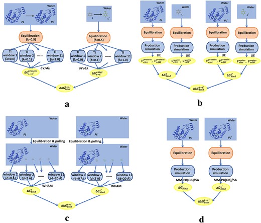
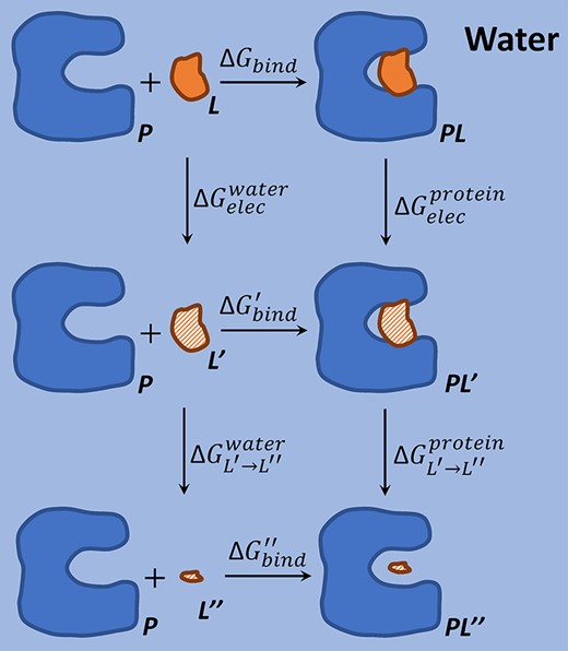
Different diagrams for calculating relative binding free energy of two ligands (|$L$| and |$L^{\prime}$|) binding to a protein (|$P$|). (A) TI method. (B) LIE method. (C) Umbrella sampling method. (D) Molecular mechanics Poisson-Boltzmann (generalized Born)/surface area (MM-PB(GB)/SA) method.
Machine learning-based scoring functions
Benchmark databases
Developing a trustworthy scoring function requires a set of protein–ligand complexes, with experimentally determined structures and affinities of high quality, for calibrating the parameters in the function. The size and quality of this set will affect the calibration or even bias the results. Efforts have been made in the past two decades to develop comprehensive databases of protein–ligand complexes, by consolidating information, such as the structural and binding data, from different sources. Below, we list a number of highly accessed databases, upon which both generic scoring functions and family-specific functions can be developed.
BindingDB: Launched in 2000 (http://www.bindingdb.org) and with a few updates thereafter [16, 30], BindingDB has collected over 1.8 million data entries of experimental protein–ligand interaction data mostly from scientific publications and patents. Drug targets or the potential candidates, coupled with small drug-like molecules, are the main focus of BindingDB. With the rapid expansion of BindingDB, currently the collected entries have covered over 7000 protein targets and 0.8 million ligands. Aside from the affinity measurements (|$K_d$|, |$K_i$| or |$IC_{50}$|), key experimental conditions (e.g. temperature, pH and buffer composition) have also curated for each entry. These entries have additionally been navigated to data sources such as the PDB, pathway databases and compound databases, according to data availability. Users can download the queries upon a free registration in the format of SDfile or TSV file, or access the database programmatically (e.g. RESTful API). BindingDB also provides a series of data sets, such as those validation sets designed for evaluation and parameterization of models in computer-aided drug design, for specialized uses.
PDBbind: PDBbind or PDBbind-CN (http://www.pdbbind.org.cn) was first released to the public in 2004 and updated annually until recently (newest release of version 2019) [114]. Differing from BindingDB, PDBbind aims to provide a solid link between molecular structural information and binding data. It was developed based on PDB, by screening for complexes of interests (e.g. protein–ligand complexes) and scraping the binding data from relevant references (|$K_d$|, |$K_i$| or |$IC_{50}$| value, preferably in a standard or near-standard experimental setting). Currently, PDBbind has covered over 21 000 biomolecular complexes, where around 18 000 are protein–ligand complexes. Additionally, the developers have filtered the collected data into a refined set by multi-step quality control and further condensed it into a core set by clustering the complexes using protein similarity, both of which have served as convenient entries into molecular docking and structure-based scoring of molecular binding affinities. Users can download the structural files together with the binding data as a package upon a free registration.
Binding MOAD: Originally published in 2005 [40] and with regular updates, Binding MOAD is a database storing high-quality, experimentally determined, structural and binding data of protein–ligand complexes (http://bindingmoad.org). Quite similar to PDBbind, Binding MOAD was developed using a top-down procedure that started from the PDB. The entry criteria for Binding MOAD include a higher resolution (|$<2.5\mathring{A}$|) of the crystal structure of the complex, at least one protein chain, a ligand that non-covalently binds to the protein, and valid binding data (|$K_a$|,|$K_d$|, |$K_i$| or |$IC_{50}$| value, order of preference: |$K_d>K_i>IC_{50}$|) curated from literature. Redundancy was further addressed by sequence alignment coupled with unified binding sites, and similarity data for the ligands and binding sites were also supplied as a part of the database. Currently, Binding MOAD (release of 2018) contains |$\sim $| 36 000 protein–ligand structures, where over 17 000 unique ligands and more than 13 000 binding data are uncovered. Binding MOAD provides different subsets from PDBbind for specialized applications, and such data can be downloaded as a package.
CSAR benchmarks: The community structure activity resource (CSAR) aims to collect high-quality data from industry and academia and make them publicly available for development and benchmarking of computational methods for ligand docking and scoring (http://www.csardock.org). The dataset released in the 2010 CSAR benchmark exercise [26] was developed for effective evaluation of different docking and scoring methods. Starting from Binding MOAD and PDBbind, two initial datasets with PDB structures deposited before 2006 (set 2) and between 2007 and 2008 (set 1) were identified. Under a series of refining processes according to high structure quality, ligand validity, preferable binding data and manual inspection, the pruned datasets were released as the CSAR high-quality (CSAR-HiQ) sets. Later with a remediation based on improved quality-assessment criteria and a further refinement work by the National Research Council of Canada (NRC), the CSAR-NRC HiQ sets (set 1: 176 complexes, set 2: 167 complexes) were released. The benchmark exercise continued annually from 2012 to 2014, with more data collected from the industry and a focus on target-specific docking/scoring [14, 25, 93]. Another major data set of CSAR, named CSAR 2012 set, was released in 2012 and covered 6 protein targets with 647 compounds and 82 crystal structures [25]. Although not all protein–ligand crystal structures were available in this set, it still serves as a valuable data source for the prediction of binding affinity (generic or target-specific). Details of all the datasets adopted for the benchmark exercises (CSAR-HiQ and CSAR 2012|$\sim $|2014) can be downloaded from the CSAR website.
Platinum: Platinum, publicly accessible at http://structure.bioc.cam.ac.uk/platinum, is a specialized database that aims at studying the effects of structural mutations on protein–ligand affinities [86]. It started with a search of valid triplets, each containing a wild-type (WT) protein, a mutant and a ligand, from PubMed articles and the PDB. The entry criteria include the release of crystal structures of the complexes (WT-ligand, mutant-ligand or both) and valid binding data for both the complexes (|$K_d$|, |$K_i$| or |$K_m$|). For each pair of WT-ligand and mutant-ligand complexes, the binding affinities were measured under the same experimental conditions by the same technique. Aside from the structural and binding data, the experimental conditions coupled with a number of ligand properties have also been supplied by Platinum. Although lacking regular updates, this database currently covers over 1000 triples and can potentially be developed into a benchmark for predicting relative biding affinities.
Scoring functions
Upon characterizing a protein–ligand complex as a set of features relevant to the binding affinity, machine-learning techniques can reveal the nonlinear relationship between such features and the binding affinity (generally log-transformed as |$pK_{d/i}=-log\ K_{d/i}$|). In the evaluation of prediction performance, Pearson’s correlation coefficient (|$R=\frac{cov(\boldsymbol{y}^{true},\boldsymbol{y}^{prediction})}{\sigma (\boldsymbol{y}^{true})\sigma (\boldsymbol{y}^{prediction})}$|), mean absolute error (|$MAE=\frac{1}{N}\sum \limits _{n=1}^{N}|y^{true}_n-y^{prediction}_n|$|) and the root mean square error (|$RMSE=\sqrt{\frac{1}{N}\sum \limits _{n=1}^{N}(y^{true}_n-y^{prediction}_n)^2}$|) are commonly used metrics. A higher correlation and a lower error indicate a better performance. In what follows, we briefly describe a number of scoring models, grouped according to different feature representations, for the prediction of protein–ligand binding affinity.
Geometrical descriptors
RF-SCORE: RF-SCORE is among the earlier studies of machine learning-based scoring functions that showed a better performance than classical scoring functions [5]. Based on a selected group of heavy-atom types |$\boldsymbol{A}=\{C,N,O,F.P,S,Cl,Br,I\}$|, the counts for interacting atom pairs (|$i$| and |$j$|) with a specific atom-type pair (|$A_p$| and |$A_l$|), expressed as |$c_{(A_p,A_l)}=\sum _{i=A_p}\sum _{j=A_l}I_{d_{ij}<d_{cut}}$|, were obtained. The interacting atoms, between the protein and ligand, were defined as pairs of atoms within a specific distance threshold (|$d_{cut}=12\mathring{A}$| in [5]). The feature set is accordingly the counts for all atom-type pairs, as |$\boldsymbol{x}=\{c_{(A_p,A_l)}|A_p\in \boldsymbol{A}, A_l\in \boldsymbol{A}\}$|. Random forests (RFs) were employed as a regression tool to map such features of each complex (|$\boldsymbol{x}_n$|, |$n=1,\ldots ,N$|) to its binding affinity (|$y_n$|, |$n=1,\ldots ,N$|). The predicted RF-SCORE can be derived by averaging the predictions from multiple trees (|$T_p$|, |$p=1,\ldots ,P$|;|$P=500$| in [5]), as |$f_{\boldsymbol{RF-SCORE}}(\boldsymbol{x})=\frac{1}{P}\sum _{p=1}^{P}T_p(\boldsymbol{x})$|. RF-SCORE was trained on the refined set of PDBbind (version 2007, with the core set excluded) and validated on the core set (|$R=0.776$| and |$RMSE=1.58$|).
Occurrences of atom-type pairs: The occurrences of atom-type pairs were also considered as features in an earlier study [23], while with a larger atom-type group (|$\boldsymbol{A}=\{C.3,C.2,C.ar,C.cat,N.3$||$,N.ar,N.am,N.pl3,$||$O.3,O.2,O.co2,F.P.3,S.3,Cl,Br,Ca,Zn,Ni,Fe\}$|) and several distances bins (|$1\mathring{A}-6\mathring{A}$| at an interval of |$1\mathring{A}$|) instead of a single threshold. After a feature-selection step, the kernel-partial least square (K-PLS) regression was applied to map these features to the binding affinities, with the radial basis function kernel used for distance calculation. As report in this work, a pruned descriptor set rather than the full set allowed |$R^2$| to reach 0.6. However, it has not been validated on a well-recognized benchmark set.
Quasi-fragmental descriptors: In another earlier work of Artemenko’s [4], such occurrences of atom-type pairs in multiple distance bins were named as quasi-fragmental descriptors. Specifically, these descriptors were extracted based on the atom types from Amber force field and a number of intervals (|$0.5\mathring{A}$|, |$1\mathring{A}$|, |$1.5\mathring{A}$|) for cutting distance bins (|$<6\mathring{A}$|), with the overlapping bins included or excluded. Besides, another group of physico-chemical descriptors (close contacts, metal-ligand interactions, flexible bonds, vdW interaction energy and electrostatic interaction energy) were included to complete the initial feature set. With a pruning of this feature set, an ensemble model of shallow neural networks was developed for a regression analysis, resulting in an average performance of |$R=0.7625$| and |$RMSE=1.79$| for a test set. Interestingly, the descriptors that frequently survived from the pruning process were primarily quasi-fragmental but not physico-chemical, demonstrating the validity of these simple geometrical descriptors in this prediction work. This method has not been validated on a well-recognized benchmark set.
CScore: In the work of Ouyang et al.[82], the atom-type pairs were further classified as repulsive or attractive by two fuzzy membership functions. These membership functions softened the boundary between repulsion and attraction for each atom-type pair, with the initial boundary defined as the sum of vdW radii of the two component atoms. Then, the occurrences of repulsive and attractive atom-type pairs were counted (|$\{c_{(A_p,A_l)}^{repulsive},c_{(A_p,A_l)}^{attractive}|A_p\in \boldsymbol{A}^P, A_l\in \boldsymbol{A}^L\}$|) and constituted the primary features in this work. Different atom types were considered for the ligand (|$\boldsymbol{A}^L=\{H,C,N,O,F,P,S,Cl,Br,I\}$|) and the protein (|$\boldsymbol{A}^P=\{H,C,N,O,S\}$|). Neural network models were employed to map the features to the binding affinities. CScore was trained on the PDBbind core set (version 2009) and tested on the refined set (with core set excluded), which had a performance of |$R=0.7668$| and |$RMSE=1.454$|.
Knowledge-based descriptors
(i) |$d_{cut}=12\mathring{A}$|
(ii)
$$\Delta d=\begin{cases}2\mathring{A},\ d\le 2\mathring{A}\\0.5\mathring{A},\ 2\mathring{A}<d\le 8\mathring{A}\\1\mathring{A},\ d>8\mathring{A}\end{cases}$$(iii) |$\boldsymbol{A}^L=\{C.3,C.2,C.ar,C.cat,N.4,N.am,N.pl3,N.2,O.3,O.2,O.co2,$||$ P.3,S.3,F,Cl,Br,I\}$|
(iv) |$\boldsymbol{A}^P=\{C.3,C.2,C.ar,C.cat,N.4,N.am,N.pl3,N.2,O.3,O.2,O.co2,$||$P.3,S.3,metals\}$|.
Such pairwise potentials were used as descriptors in different scenarios for protein–ligand binding, and then absorbed by support vector regression (SVR) models to predict the binding affinity. This SVR-KB score was trained on the PDBbind refined set (version 2010) and tested on the CSAR-NRC HiQ sets, leading to the performances of |$R=0.67$| (set 1) and |$R=0.59$| (set 2).
Physico-chemical descriptors
SVR-EP score: In the work of Li et al.[66], a group of physico-chemical descriptors were considered in the binding affinity prediction. These descriptors included ligand molecular weight, vdW interaction energy, hydrogen bonds, ligand deformation effects (rotatable bonds), hydrophobic effects and several terms concerning the SASA (buried/unburied, polar/nonpolar and ratios). Upon a feature selection step, the remaining descriptors were adopted by SVR models for binding affinity prediction. This SVR-EP score was trained on the PDBbind refined set (version 2010) and tested on the CSAR-NRC HiQ sets, with the performances of |$R=0.55$| (set 1) and |$R=0.50$| (set 2).
B2BScore: Liu et al.[69] developed the B2BScore by exploring two physical–chemical properties (B factors and |$\beta $| contacts) and learning them through RF regression models, in order to predict protein–ligand binding affinity. B factor quantifies the mobility of an atom in a dynamic protein structure, and a larger value generally suggests a higher flexibility of the atom. A normalized form of B factors for each atom was used in (|$\hat{B}_i\in [0,2]$|) [69]. A |$\beta $| contact between atoms |$i$| and |$j$|, defined upon a distance threshold (|$d_{cut}=2.8\mathring{A}$| in [69]) and an angle threshold (|$\angle \beta \in [75,90]$|, depending on |$d_{ij}$| in [69]), guarantees a forbidden region for enough direct contact between |$i$| and |$j$| (no other atoms in this region). A |$\beta $|-contacts graph can be constructed for a given protein–ligand complex, with each point representing a heavy atom and each edge a |$\beta $| contact. Depending on the |$\beta $|-contacts graph, a series of descriptors were generated based on the B factors of involved atoms. These descriptors characterized the cross-interface |$\beta $| contacts (for each atom-type pair), the within-binding-site |$\beta $| contacts (for each atom-type pair), the |$\pi $|-center involved |$\beta $| contacts, the backbone-atom involved |$\beta $| contacts, the metal-ion involved |$\beta $| contacts, the interacting atoms in ligand and the interfacial backbone atoms. Later, the descriptors were adopted by RFs for the prediction of binding affinity. B2BScore was trained on the PDBbind refined set (version 2009, with core set excluded) and tested on the core set, outperforming a number of scoring functions with |$R=0.746$| and |$RMSE=1.593$|. It was also tested under the leave-one-cluster-out cross-validation scheme by grouping the proteins into 26 clusters in the PDBbind refined set, and it outperformed the RF-SCORE with |$\bar{R}=0.518$|.
ID-Score: Li et al.[65] developed ID-Score by involving 50 descriptors relevant to protein-ligand interactions and employing SVR models for affinity prediction. Those 50 descriptors, mostly physico-chemical, were classified into nine categories. Specifically, the descriptors characterized the vdW interactions ascribed to different atom-type pairs, the hydrogen-bonding interactions for a number of acceptor–donor pairs, the electrostatic interactions, the |$\pi $|-system interactions (|$\pi $|-|$\pi $| interactions, halogen-|$\pi $| interactions and electronegative atoms-|$\pi $| interactions), the metal-ligand interactions (O/N atoms in ligand with metal cations), the desolvation effects concerning the ligand (hydrophilicity, polar surface area, volume and SASA) and protein (ratio of the polar surface area to the non-polar surface area of the protein binding pocket, and the binding-site SASA), the entropy effects concerning ligand rotatable bonds, the shape complementarity between a ligand and its target and the property complementarity between the ligand surface and the binding-site surface (ascribed to electrostatic-property pairs). SVR models based on these descriptors were trained on the PDBbind refined set (version 2011, with core set excluded) and tested on the core set, with the performance of |$R=0.7525$| and |$RMSE=1.6282$|. Besides, ID-Score also performed well in target-specific predictions, with |$R$| ranging from 0.627 to 0.851 (|$\bar{R}=0.764$|) for a carefully collected test set covering 20 diverse targets.
SFCscore|$\boldsymbol{^{RF}}$|: In the work of Zilian et al.[124], the conjunction of a rich set of descriptors developed earlier [95] and RF regression models evolved into the efficient |$\boldsymbol{SFCscore^{RF}}$| for the prediction of protein–ligand binding affinity. These descriptors are mostly physico-chemical and were also used in the construction of SFCscore[95]. In details, they described the simple ligand characteristics (molecular weight and number of atoms), the hydrogen bonds and scores (total number, total score, scores of charged and neutral hydrogen bonds), the metal-ligand interactions, the aromatic ring interactions (ring-ring, ring-metal and ring-lysine side chain), the hydrophobic effects (complementarity between the protein and ligand, and percentage of buried carbon atoms of the ligand), the entropy effects concerning rotatable bonds and scores (total number, total score and score of |$sp^3-sp^3/sp^2$| bonds) and the properties (hydrophobic, polar and aromatic) of several types of surfaces (total, buried, exposed and contact surfaces of the ligand and protein). By training RF regression models on the PDBbind refined set (version 2007, with the core set and CSAR-NRC HiQ sets excluded) using such descriptors, the derived |$\boldsymbol{SFCscore^{RF}}$| achieved the performances of |$R=0.779/RMSE=1.56$| and |$R=0.730/RMSE=1.53$| on the core set and CSAR-NRC HiQ set (combining sets 1 and 2), respectively. Applying |$\boldsymbol{SFCscore^{RF}}$| to several target-specific prediction tasks also achieved a good performance.
Proteochemometric characterization
Proteochemometric approaches, first proposed by Wikberg et al.[61], indicate using structural features of both the protein (the binding site and neighborhood) and the ligand in the construction of predictive models.
PESD signatures: On the basis of the proteochemometric concept, Das et al.[20] developed the property-encoded shape distribution (PESD) signatures for protein–ligand interaction surfaces, which were used as features by SVR models for binding affinity prediction. The protein interaction surface (PIS) and ligand interaction surface (LIS) for each complex were defined based on distance cutoffs for protein–ligand atom pairs (|$4.5\mathring{A}$| for PISs and |$3\mathring{A}$| for LISs). These PISs and LISs were further encoded with physico-chemical properties by EP (electrostatic potential) and ALP (hydrogen bonds, polarization and hydrophobicity) surface maps [60]. In total, 100 000 point pairs with various distances on a property-encoded interaction surface (PIS or LIS), which was triangulated for simplicity, were sampled. Specifically, the distance was binned (|$\boldsymbol{D}=\{[0,1\mathring{A}],[1\mathring{A},2\mathring{A}],\ldots ,[23\mathring{A},24\mathring{A}]\}$|) and the property magnitudes were coarse-grained into several bins (9 for EP properties: |$\boldsymbol{P}^{EP}=\{P^{EP}_1,\ldots ,P^{EP}_9\}$| and 14 for ALP properties: |$\boldsymbol{P}^{ALP}=\{P^{ALP}_1,\ldots ,P^{ALP}_{14}\}$|). Each point pair was assigned to a two-dimensional bin, with the bin populations (|$\{c_{d,(p_1,p_2)}^{EP}|d\in \boldsymbol{D},p_1\in \boldsymbol{P}^{EP},p_2\in \boldsymbol{P}^{EP}\}$| or |$\{c_{d,(p_1,p_2)}^{ALP}|d\in \boldsymbol{D},p_1\in \boldsymbol{P}^{ALP},p_2\in \boldsymbol{P}^{ALP}\}$|) counted. Such bin populations regarding the EP and ALP properties for both the PIS and LIS, |$\{c_{d,(p_1,p_2)}^{EP,PIS}, c_{d,(p_1,p_2)}^{EP,LIS}, c_{d,(p_1,p_2)}^{ALP,PIS}, c_{d,(p_1,p_2)}^{ALP,LIS}\}$|, constituted the PESD signatures for a protein–ligand complex and were fed into an SVR model for affinity prediction. This method was trained on the PDBbind refined set (version 2005, with the core set excluded) and tested on the core set, yielding a better prediction performance of |$R=0.638/MAE=1.45$| compared with classical empirical scoring functions.
QSAR descriptors: Machine-learning approaches have been extensively applied to decoding quantitative structure-activity relationships (QSAR) [34]. The QSAR bioactivity predictions primarily focus on ligand-only properties/signatures (e.g. extended-connectivity fingerprints (ECFPs) [89]), protein-only features (mostly of amino acid sequences, e.g. amino acid composition descriptors and autocorrelation descriptors) and any combinations thereof. This differs from typical machine learning-based scoring functions in exploiting the protein structures or protein–ligand relative structures. (i) In the work of Li et al.[67], QSAR descriptors for the protein sequence, the ligand and the binding pocket (e.g. charged partial surface area) were adopted in the prediction of protein–ligand binding affinity. This method can also be considered as proteochemometric, although the proteins were characterized using the sequence properties instead of structural features. The initial 3286 descriptors were pruned by checking the redundancy and weighting the relevance to the target, upon which the least squares support vector machines were employed for a regression analysis. Two separate models were built for predicting |$K_d$| and |$K_i$| affinities in the PDBbind refined set (version 2007). For |$K_d$| or |$K_i$| samples in this set, the training and testing samples were partitioned as |$4:1$|. The testing performances of |$R=0.833/RMSE=1.118$| and |$R=0.742/RMSE=1.471$| were derived in the two scenarios. However, the cutoffs for redundancy checking and relevance weighting in this work seem quite arbitrary, and the resulting descriptors may in turn bias the prediction performance. (ii) In another work of Kundu et al.[60] that adopted a similar proteochemometric concept, features describing the whole protein and the ligand were extracted for a set of protein–ligand complexes (a subset of PDBbind of version 2015), upon which machine-learning methods such as RFs were trained. In detail, descriptors of the proteins included the amino acid compositions of the sequence, SASA, hydrogen bonds for describing different secondary structures, number of chains, number of |$S-S$| bridges and number of residues. For ligands, the atom counts for different atom types, bound types and ring types and a number of physico-chemical properties (e.g. molecular weight and hydrogen-bond accepor/donor) were considered. The 10-fold cross-validation performance on the PDBbind subset reached |$R^2=0.765/RMSE=1.31$|, and the performance of a blind-set validation (|$4:1$| for training and testing samples in the PDBbind subset) achieved |$R^2=0.75/RMSE=1.38$|.
PLEC fingerprint: W|$\acute{o}$|jcikowski et al.[118] proposed the protein–ligand extended connectivity (PLEC) fingerprint to encode protein-ligand interactions, and employed such fingerprints in the construction of machine-learning models tailored for binding-affinity prediction. PLEC fingerprints belong to the QSAR community, and the related predictive models are proteochemometric as they adopt the fingerprints of fragments from both the protein and ligand. In the generation of PLEC fingerprints, interacting atom pairs were first identified (|$d_{ij}<4.5\mathring{A}$|) with |$n$|-depth neighborhoods of each atom defined, and then pairings between the ligand and protein atomic neighborhoods based on depth thresholds (|$n^P$| for protein and |$n^L$| for ligand) were conducted with each pairing hashed to a bit position in the PLEC fingerprint. The following depth pairs of the ligand and protein atomic neighborhoods were used in the pairings.
|$\{(n^p,n^l)|n^p=n^l\le \min (n^P,n^L)\}$|
- $$\{(n^p,n^l)|\begin{cases}n^l=n^L,n^L<n^p\le n^P;\ \ \ n^L<n^P\\ n^p=n^P,n^P<n^l\le n^L;\ \ \ n^P<n^L\end{cases}\}$$
These atomic neighborhoods were encoded by the ECFPs, which concern the features of atomic number, isotope, number of neighboring heavy atoms, number of hydrogen atoms, formal charge, ring membership and aromaticity [89]. Later, a raw PLEC fingerprint was folded to a smaller length. Comparisons among the PLEC fingerprints can be relied on common similarity measures such as the Tanimoto coefficients. Using these PLEC fingerprints, machine-learning models were trained on the PDBbind general set (version 2016, with the core set and Astex diverse set [38] excluded), with the neighborhood depths (|$n^P$| and |$n^L$|) and fingerprint folding size tuned. The best models yielded promising prediction results on the core set (|$R=0.817$|) and the Astex diverse set (|$R\in [0.65,0.7]$|), outperforming a number of other approaches. A similar structural protein–ligand interaction fingerprint (SPLIF), which was developed earlier with |$n^P=n^L=1$|[18], also resulted in a good affinity prediction in PDBbind[119].
Featurizers tailored for deep-learning methods
Traditional machine learning-based scoring functions rely heavily on representing molecules with hand-curated, fixed-length vector features. This limitation can be mitigated by the flexibility of deep neural networks, which make data-driven decisions to learn a hierarchy of feature representations from the simplest representations. Recently, such deep-learning models have begun to thrive in the fields of computational biology, chemistry and physics, including the studies of protein–ligand binding [33]. Below, we list several promising deep-learning models that have been applied to the prediction of protein–ligand binding affinity.
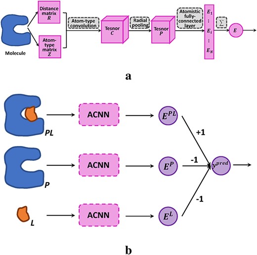
The architecture of ACNNs and the application to protein–ligand (|$P-L$|) affinity prediction. (A) ACNN architecture. (B) Combining ACNNs with a thermodynamic cycle for affinity prediction.
|$\boldsymbol{K_{DEEP}}$|: In [50], |$\boldsymbol{K_{DEEP}}$|, which integrated 3D voxel representations of molecules and 3D convolutional neural networks (CNNs), was developed to predict protein–ligand binding affinity. The voxel representation indicates a 3D-grid featurizer, where each voxel or grid point is described by the properties (e.g. atom type or physico-chemical types) of the atoms nearby. A 3D-grid of a fixed size (|$24\mathring{A}\times 24\mathring{A}\times 24\mathring{A}$| with |$1\mathring{A}$| intervals at each side in [50]) is generally placed at the geometric center of the ligand, in order to capture a neighborhood of the binding site. The atomic properties including hydrophobicity, hydrogen-bond donor and acceptor, aromaticity, positive ionizable or negative ionizable, metallicity and excluded volume for both the protein and ligand in a complex were considered in [50], leading to 16 channels in the representation. Such a voxel representation can be summarized as a 4D-tensor |$(x,y,z,(f_1,\ldots ,f_{16}))$|, where the first three dimensions indicate the Cartesian coordinates of the center of a voxel and the last dimension is a vector of properties describing this voxel (Figure 7). In each property channel, the contribution of an atom to a voxel is measured according to the vdW radius |$r_{vdW}$| of this atom and the atom-voxel distance |$r$|, as |$n(r) = 1-exp(-(\frac{r_{vdW}}{r})^{12})$|. To train a model insensitive to protein–ligand orientation, each complex structure was augmented to 24 structures with different orientations by rotated 3D-grids (all possible combinations of 90|$^{\circ }$| rotations). The 3D CNNs, comprising multiple convolutional/pooling layers and a fully connected layer, were applied to the learning of such representations. The network architecture was initially inspired by AlexNet [44]. |$\boldsymbol{K_{DEEP}}$| was trained on the PDBbind refined set (version 2016, with the core set excluded) and tested on the core set, having a performance of |$R=0.82/RMSE=1.27$|. It was also tested on a number of other benchmarks such as the CSAR sets, resulting in superior or competitive performances compared with other predictions.
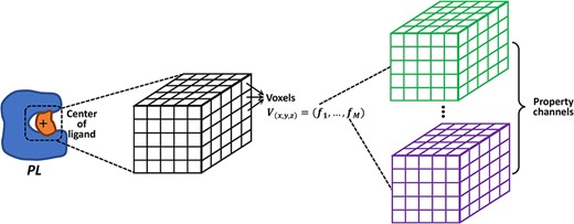
Voxel representation focused on the geometrical center of the ligand in a protein-ligand complex, with |$M$| property channels.
Pafnucy: Stepniewska-Dziubinska et al.[98] developed Pafnucy, a similar model to |$\boldsymbol{K_{DEEP}}$| that uses CNNs to process voxel representations of protein–ligand complexes for affinity prediction. In their study, each complex was cropped to a cubic box with the size of |$20\mathring{A}\times 20\mathring{A}\times 20\mathring{A}$| and the focus at the geometric center of the ligand. A 3D-grid was generated for the cubic box with |$1\mathring{A}$| spacing, and all heavy atoms were placed in the grids by discretizing their positions, differing from |$\boldsymbol{K_{DEEP}}$| that measures the contributions of each atom to each grid point. Pafnucy covers more atomic properties, including nine atom types, atom hybridization, bonds to heavy atoms, bonds to other heteroatoms, hydrophobicity, aromaticity, hydrogen-bond donor and acceptor, ring membership, partial charge and the sign for protein/ligand. The properties for each voxel were derived by summing up the values of all colliding atoms in that voxel. The voxel representations were subsequently learned by CNNs, with an architecture composed of three 3D convolutional layers, each followed by a max pooling layer, and three fully connected layers, followed by a final single output neuron for predicting the binding affinity. Pafnucy was trained on the PDBbind general set (version 2016, with the validation/test sets excluded) with a validation on a random set selected from the refined set (1000 complexes) for parameter tuning. Then, the trained model was tested on the PDBbind core sets (version 2016 and 2013) and the Astex diverse set [38], with the performances of |$R=0.78/RMSE=1.42$|, |$R=0.70/RMSE=1.62$| and |$R=0.57/RMSE=1.43$|, respectively.
DeepDTA: In [83], the DeepDTA model, which describes a protein–ligand complex by a 1D representation and employs CNNs to learn these representations, was proposed for the prediction of protein–ligand binding affinity. The 1D representation was derived by a simple label encoding (64 labels for ligand and 25 labels for protein) of the ligand SMILES sequence and the protein sequence into fixed lengths (by truncation or 0-padding). Then, a network architecture composed of two convolution blocks (one for the ligand and the other for the protein) and one block of fully connected layers was adopted for processing these representations. The convolution blocks each concatenate three convolutional layers and one max-pooling layer, and the final block contains three fully connected layers (with dropouts used to avoid overfitting). DeepDTA was trained and tested on two data sets (Davis[21] and KIBA[101]), with |$\frac{5}{6}$| of each set used for training (5-fold cross-validation scheme) and |$\frac{1}{6}$| for testing. The concordance index (|$CI$|), which measures whether the predicted affinities were in the same order as the true affinities were, and mean square error (|$MSE=RMSE^2$|) were used for performance evaluation. The performances were |$CI=0.878/MSE=0.261$| (Davis set) and |$CI=0.863/MSE=0.194$| (KIBA set), respectively. However, this work has not been validated on a well-recognized benckmark or compared with other state-of-the-art scoring functions. Furthermore, the constructed models seemed dataset-specific (e.g. different dimensions for inputs), which may be questioned for the generalization capabilities to other datasets.
DeepBindRG: Zhang et al.[121] developed DeepBindRG, which uses a deep-learning model to learn protein–ligand contacts, for predicting the binding affinity. In the characterization of protein–ligand complexes, the atom types for the ligand and protein were first defined referring to the generalized Amber force field (84 types for ligand) and the Amber99 force field (41 types for protein). Protein–ligand interacting atom pairs were identified based on a distance threshold (|$4\mathring{A}$|), and the atoms in each pair were one-hot encoded according to the ligand atom types or the protein atom types. The interacting atoms in each protein were further clustered into five groups, for gathering the atom pairs that had atoms in the same group in the contact matrix |$C$|. |$C$| is the final feature representation of a protein–ligand complex, with 1000 rows (by truncation or 0-padding) and each row indicating the one-hot representation of an interacting atom pair. Clustering the protein interacting atoms seemed to retain the local spatial information, which can be useful in convolutions. Such extracted 2D features were learned by a ResNet, consisting of seven convolutional blocks (three convolutional layers for each), a max pooling layer and a fully connected layer, to predict protein–ligand binding affinity. The PDBbind general set (version 2018, with several independent test sets excluded) was partitioned for training, validation and testing of DeepBindRG, with a performance of |$R=0.5993/RMSE=1.497$| on the test set. Furthermore, the trained model was tested on several independent sets and had prediction performances of |$R=0.6394/RMSE=1.817$| for the core set (version 2013), |$R=0.6585/RMSE=1.7239$| for the CSAR-NRC HiQ set and |$R=0.4657/RMSE=1.6209$| for the Astex diverse set [38]. However, this model underperformed Pafnucy (described above) in the predictions for several test sets and lacked a thorough comparison with other state-of-the-art scoring functions.
Experimental and predicted binding free energies of small molecules binding to bacteriophage T4 lysozyme. Prediction methods include TI, LIE, umbrella sampling (US) and molecular mechanics Poisson-Boltzmann (generalized Born)/surface area (MM-PB(GB)/SA)
| Predicted |$\Delta\Delta G_{bind}^{[b]}$| (computational costs|$^{[c]}$|) | ||||||
|---|---|---|---|---|---|---|
| Ligand pair (formula) | Experimental |$\Delta\Delta G_{bind}^{[a]}$| | TI | LIE | US | MM-PB/SA | MM-GB/SA |
| benzene|$\rightarrow$|toluene (C6H6|$\rightarrow$|C7H8) | −0.32 | 0.02|$\pm$|0.14 (73.67) | −0.65|$\pm$|0.68 (3.57) | 6.05 (129.7) | −1.33|$\pm$|2.46 (3.25) | −3.09|$\pm$|1.97 (2.8) |
| benzene|$\rightarrow$|phenol (C6H6|$\rightarrow$|C6H6O) | |$>0$| | 1.35|$\pm$|0.44 (10.05) | −1.55|$\pm$|1.13 (3.58) | 7.15 (128.68) | 1.24|$\pm$|2.93 (3.26) | −0.62|$\pm$|2.20 (2.81) |
[a]Calculated based on experimental |$K_d$| values. |$\Delta \Delta G_{bind}^{L\rightarrow L^{\prime}}=RT\ ln(\frac{K_d^{L\prime}}{K_d^L})$| with |$T=300$| K.
[b] In kcal/mol. |$K_d$||$\sigma_{\Delta\Delta G_{bind}^{L\rightarrow L\prime}}=\sqrt{\sigma_{\Delta G_{L\rightarrow L\prime}^{protein}}^2\pm\sigma_{\Delta G_{L\rightarrow L\prime}^{water}}^2}$| (TI) or |$\sigma_{\Delta\Delta G_{bind}^{L\rightarrow L\prime}}=\sqrt{\sigma_{\Delta G_{bind}^{L}}^2\pm\sigma_{\Delta G_{bind}^{L\prime}}^2}$| (LIE and MM-PB(GB)/SA).
[c]In hours. Calculated as the sum of simulation time and energy-estimation time.
[d]Entropy contributions not included
Case study of interpretable scoring functions
Since many machine-learning methods involve ‘black boxes’, obtaining interpretable scoring functions is an important goal in machine learning-based affinity prediction. In this regard, we conducted a case study of several interpretable scoring functions, based on simple geometrical descriptors that have led to good prediction performance and are closed tied to a number of scoring functions (e.g. RF-Score, Quasi-fragmental descriptors, CScore, SVR-KB and ACNN). Specifically, the latest PDBbind refined set (version 2019, with the core set excluded) of 4586 protein–ligand complexes were used for training the scoring functions, and the core set (CASF 2016) of 285 complexes for validation. These datasets mostly contain drug-like ligands and a variety of protein targets, which serve as useful data sources for scoring-function development and computer-aided drug discovery. The geometrical descriptors in RF-Score (Section 4.2.1; [5]) were used to characterize each protein–ligand complex. These descriptors |$\{c_{(A_p,A_l)}\}$| (36 types) indicate the occurrences of atom-type pairs (|$A_p$|, |$A_l$|) in the interaction sites. For example, |$c_{(C,C)}$| represents the count of interacting atom pairs each comprising a Carbon atom from the protein and a Carbon atom from the ligand. Then, we used linear regression models, regression trees and RFs to map these descriptors to the experimental binding affinity (|$\Delta G_{bind}=RT\ ln(K_d)$| with |$K_d$| supplied by PDBbind and T=300 K). These models were selected because they are simpler but more interpretable than other machine-learning models like neural networks, and we name the corresponding scoring functions as LM-Score, TREE-Score and RF-Score. The tree in TREE-Score was pruned using an optimal complexity parameter that was evaluated by cross validation [102]. The setting in [5] were adopted for constructing RF-Score (500 trees, optimal number of descriptors considered at each split: 8). All the models were run in a CPU setting (Intel® CoreTM i9-9900K @ 3.60GHz).
The distributions of the selected geometrical descriptors, in the training and test sets, are displayed in Figure 8A. We can see that occurrences of atom-type pairs such as |$(C,C)$|, |$(N,C)$| and |$(O,C)$| are dominant, which makes sense since these are the commonest heavy atoms in proteins and ligands. The scoring functions were trained using these descriptors and the experimental affinity data of the training set and tested on the validation set (results in Table 2). From the computational costs (time for descriptor extraction, training and validation) listed in Table 2, we can see that these scoring functions are quite efficient. More results are elaborated as follows.
(i) LM-Score: Using the simplest linear regression model, we derived an RMSE of 2.34 kcal/mol, the correlations of 0.657 (Pearson’s) and 0.681 (Spearman’s). The detailed scoring function can be expression as |$y_{pred}=-0.0005\times c_{C,C}-0.0012\times c_{N,C}-0.0002\times c_{O,C}-0.0016\times c_{S,C}-0.0005\times c_{C,N}-0.0028\times c_{N,N}+0.0028\times c_{O,N}-0.0227\times c_{S,N}-0.0002\times c_{C,O}+ 0.0056\times c_{N,O}-0.0045\times c_{O,O}+0.0222\times c_{S,O}+0.0024\times c_{C,F}-0.0218\times c_{N,F}+0.0093\times c_{O,F}-0.0156\times c_{S,F}+0.0072\times c_{C,P}-0.0398\times c_{N,P}+0.0125\times c_{O,P}-0.0076\times c_{S,P}-0.0024\times c_{C,S}-0.0217\times c_{N,S}+0.0084\times c_{O,S}+0.1573\times c_{S,S}+0.0041\times c_{C,Cl}-0.0049\times c_{N,Cl}-0.0158\times c_{O,Cl}-0.0600\times c_{S,Cl}+0.0093\times c_{C,Br}+0.0298\times c_{N,Br}-0.0640\times c_{O,Br}-0.1271\times c_{S,Br}+0.0028\times c_{C,I}+0.0364\times c_{N,I}-0.0376\times c_{O,I}-0.1313\times c_{S,I}-5.5858$|. The predicted binding affinities are presented in Figure 9A.
(ii) TREE-Score: Compared with LM-Score, employing regression trees improved the prediction performance (RMSE=2.18 kcal/mol, Person’s and Spearman’s correlations of 0.701 and 0.705). The predicted affinities are displayed in Figure 9B, where the predicted values are stratified mainly due to the structure of the regression tree. The final pruned regression tree, as shown in Figure 9D, classifies a protein–ligand complex according to the rules in the non-leaf nodes and scores it using the value of the leaf node that it belongs to. As an instance, if a complex has descriptors of |$c_{C,C}\lt 2182$|, |$c_{N,S}\ge 68$| and |$c_{N,N}\lt 68$|, then it belongs to leaf node 13 and has the predicted binding affinity of -6.8 kcal/mol.
(iii) RF-Score: An RF comprises a group of trees with similar structures as Figure 9D. Specifically, 500 trees with each split considering eight randomly selected descriptors were constructed in this work, and each complex was scored as the averaged outputs of these trees. The importance rankings of all the descriptors in the constructed RF are shown in Figure 8B, demonstrating that descriptors like |$c_{C,O}$|, |$c_{O,O}$| and |$c_{N,O}$| primarily influenced the predictions. Using such complicated models resulted in a further improvement in the prediction performance (RMSE=1.98 kcal/mol, Person’s and Spearman’s correlations of 0.789 and 0.785).
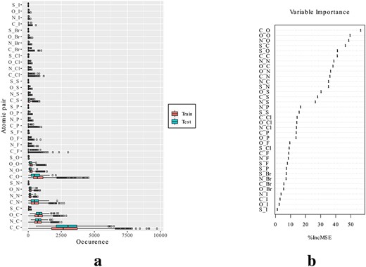
Geometrical descriptors representing the occurrences of atom-type pairs in protein–ligand interaction sites. (A) Descriptor distributions in the training and test sets. (B) Importance of descriptors in RF-Score, according to the increase in mean square error of predictions (%IncMSE) caused by permuting each descriptor.
Performance comparisons among LM-Score, TREE-Score and RF-Score. Scoring functions were trained on PDBbind refined set (2019) and tested on the core set. The predicted affinities for the core set were evaluated according to the RMSE and correlations to the experimental data, as shown below
| Scoring function | RMSE (kcal/mol) | Pearson's correlation | Spearman's correlation | Computational costs|$^{[a]}$| (minutes) |
|---|---|---|---|---|
| LM-Score | 2.34 | 0.657 | 0.681 | 1.85 |
| TREE-Score | 2.18 | 0.701 | 0.705 | 1.85 |
| RF-Score | 1.98 | 0.789 | 0.785 | 19.70 |
| Scoring function | RMSE (kcal/mol) | Pearson's correlation | Spearman's correlation | Computational costs|$^{[a]}$| (minutes) |
|---|---|---|---|---|
| LM-Score | 2.34 | 0.657 | 0.681 | 1.85 |
| TREE-Score | 2.18 | 0.701 | 0.705 | 1.85 |
| RF-Score | 1.98 | 0.789 | 0.785 | 19.70 |
[a]Computational costs include the time for descriptor extraction, training and validation.
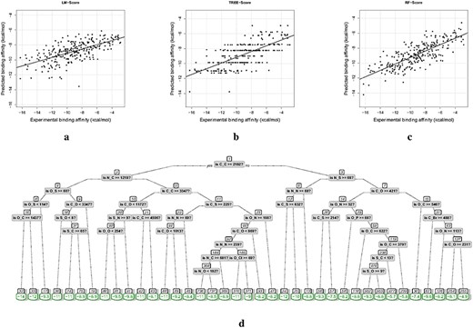
Prediction results. Experimental versus predicted binding affinities by (A) LM-Score, (B) TREE-Score and (C) RF-Score. (D) The tree structure of TREE-Score.
Fusion and choice
Free energy-based simulations and machine learning-based scoring functions are two different groups of methods. Simulation methods mainly depend on thermodynamic-cycle designing, free-energy sampling and MD simulations (MM, QM or hybridization). MD simulations are often used to capture dynamical processes of biomolecules across different timescales, generating large amount of data (compressed as trajectory files). These data provide a valuable source of information for predicting free-energy differences in simulation methods, while are rarely used in machine learning-based scoring functions. The scoring functions mostly consider single, static complex structures and are constructed primarily based on characterizing the ligand-binding pockets. Modern GPU calculations have made the MD simulations much more efficient, offering an opportunity for fusion with machine-learning methods in constructing predictive models. For binding-affinity prediction in protein–ligand complexes, using the knowledge extracted from the rich simulation data to build scoring functions will be a promising direction in near future [85, 107].
Besides potential fusions between the two groups of methods, choice between them is another important topic. Compared with other free energy-based simulations, the MM-GB/SA method only depends on end-state simulations (|$LP$| in water) and is therefore considered as an efficient simulation method. Accordingly, we attempted to compare MM-GB/SA with several scoring functions (in Section 4.3) in a case study. A small set of 100 protein–ligand complexes were used for validation (listed in Supplementary Table 1). It stemmed from the PDBbind core set (CASF 2016), and was further purified by removing complexes with crystal structures that have gaps (missing or modified residues) or metal interactions. Such selections aimed for faster and more accurate simulations. Specific settings for the methods are listed as follows.
(i) MM-GB/SA: For the simulations of each complex, a short energy minimization (500 steps), a heating step (50 ps), an equilibration step (500 ps) and a production simulation (3 ns) were conducted (same as in Section 3.5). The first 1-ns simulation data were abandoned and the following 2-ns trajectories (100 frames) were used for the calculation of binding free energy. Mostly, MM-GB/SA is employed for calculating the effective part of binding free energy (|$\Delta \tilde{G}_{bind}$|), namely ignoring the entropy contribution that is difficult to estimate. Although methods such as NMA can be used for entropy estimation, combining the effective part and such an estimated entropy may not lead to a better prediction of the absolute binding free energy. To provide a comparison with |$\Delta \tilde{G}_{bind}$|, we estimated the binding free energy with entropy contribution for each complex. Only 20 trajectory frames were used for this estimation, due to the high computational costs of NMA calculations. All the simulations were GPU-accelerated, but the MM-PB/SA and NMA calculations were implemented using 20 CPU parallel processes (GPU-calculations not available).
(ii) Scoring functions: The machine learning-based scoring functions were also validated on the above-mentioned 100 complexes, while trained on the remaining complexes in the core set. Here, the information of validation set was not used when constructing the scoring functions, which differed from the simulation methods. Besides, the training set contained some complexes with gapped structures, which may not make a large difference as the scoring functions mostly concern the protein–ligand interaction sites (structural gaps rarely occur). TREE-Score was constructed as a pruned tree (with the optimal complexity parameter), and RF-Score was built using 20 trees (due to the small set) and considering 24 descriptors at each split. All the models were run in a CPU setting (same as in Section 4.3).
Since MM-GB/SA only calculates |$\Delta \tilde{G}_{bind}$|, we evaluated the methods using correlations between the predicted and experimental affinities. The results are shown in Table 3. The |$\Delta \tilde{G}_{bind}$| calculated by MM-GB/SA achieved a correlation of |$>0.6$| with the experimental affinities, which outperformed or was comparable to the scoring functions. However, adding the entropy contributions (NMA-estimated) did not improve the correlations between the predicted and experimental affinities (|$>0.5$|). Using more data for entropy estimation or employing other estimation strategies may improve the results, but it remains a challenge. On the other hand, it indicates that MM-GB/SA is more applicable to calculating the relative binding affinities of similar systems. The simulations and MM-GB/SA predictions costed |$\sim $|297 hours (without entropy) and |$\sim $|616 hours (with entropy) for the selected complexes, which were much more expensive than the scoring functions (costs of several seconds). However, it is worth noting that, the scoring functions performed worse than those in Section 4.3 (with more training data), which demonstrated their strong dependence on training data. Conversely, it also shows that such scoring functions are improvable upon increased quantity/quality of training data. Using more data will not improve the performance of simulation methods primarily due to their latent physical models. The best performer in scoring functions (RF-Score) corresponded to correlations of 0.65 (Person’s) and 0.612 (Spearman’s) between the predicted and experimental data, which was comparable with MM-GB/SA with no entropy estimation (Person’s correlation: 0.627, Spearman’s correlation: 0.616). Methods like FEP/TI and umbrella sampling are promising to offer more accurate predictions, but with much higher computational costs. Overall, free energy-based simulations are commonly applicable to small-scale, accurate calculations of relative binding affinities, whereas machine learning-based scoring functions are improvable with more data and can be used efficiently for large-scale predictions of absolute binding affinities.
Discussion and conclusion
Free energy-based simulations and machine learning-based scoring functions are capable of providing accurate predictions of protein–ligand binding affinity. These two classes of computational methods have their specific strengths. Free energy-based simulations mostly consider the physical processes in molecular recognition, have a sound basis in statistical mechanisms and do not depend on a heavy parametrization. Based on the rapid growth of data available from the chemical and crystallographic communities, machine learning-based scoring functions are data-driven, can implicitly capture the binding effects that are hard to be modeled explicitly and can fast screen a vast number of compounds. Aside from these strengths, they also have some weaknesses as follows.
To achieve chemical accuracy in molecular simulations, the bottlenecks are the underlying physical models and the sampling convergence [49]. The sampling problem is the most important in this scenario, and the simulations hold great promise if the sampling convergence is solved. Technically, sampling difficulty in the simulations can be tackled with better algorithms and more powerful computers. A number of enhanced sampling methods (e.g. replica exchange [100], orthogonal space tempering [122], REST [68] and REST2 [112]) have been proposed accordingly. With the advances in such enhanced sampling techniques and the GPU-accelerated simulations, the sampling problem can be greatly mitigated. Compared with the sampling errors, the force-field errors are most likely small but fundamental. Progress has also been made in this field to support accurate simulations. Modern accurate force fields (e.g. OPLS3 force field [37] and polarized force fields [49, 117]) have been broadly applied in the simulations. Overall, these modern techniques have aided the accurate free energy-based simulations for affinity prediction. Nevertheless, there is still room for improvements in these techniques. Additionally, such simulations are computationally very expensive and remain impractical for the screening of a large number of protein–ligand complexes. Typically, they are limited to family-specific predictions [5].
Performance comparison between free energy-based simulations (MM-GB/SA) and machine learning-based scoring functions (|$\textbf{LM-Score}$|, |$\textbf{TREE-Score}$| and |$\textbf{RF-Score}$|). Performance was validated on a high-quality data set of 100 protein--ligand complexes, according to the correlations between predicted and experimental affinities
| Method | Pearson's correlation | Spearman's correlation | Computational costs[a] | |
|---|---|---|---|---|
| Free energy-based simulations | MM-GB/SA (no entropy) | 0.627 | 0.616 | 297.43 hours (2.97 hours per complex) |
| MM-GB/SA(with entropy[b]) | 0.534 | 0.526 | 616.20 hours (6.51 hours per complex) | |
| LM-Score | 0.529 | 0.594 | 8 seconds | |
| Machine learning-based scoring functions | TREE-Score | 0.557 | 0.568 | 8 seconds |
| RF-Score | 0.65 | 0.612 | 8 seconds |
[a]Computational costs for MM-GB/SA include the time for simulations and free-energy calculations, costs for scoring functions include the time for descriptor extraction, training and validation.
[b]Entropy contributions were estimated using the NMA.
Developing a machine learning-based scoring function, which is generally structure-guided, depends heavily on the quality of data for learning and the featurizer for representing the protein–ligand complexes. Considerable efforts have been made in the past two decades to construct comprehensive benchmark databases for the development and evaluation of scoring functions. Although it is hard to define a perfect data set, some common characteristics include high-resolution structures, a wide range of protein targets with each having several congeneric series of ligands (drug-like, both actives and inactives included), valid experimental affinity, consistency across the experiments for targets and the inclusion of experimental values of ligand physical properties [26]. Given a dataset, a generic scoring function is often learned from all the protein targets with different experimental techniques and affinity measurements (|$K_d$|, |$K_i$| and |$IC_{50}$|). However, this generic treatment may increase the noise in the affinity prediction. Moreover, the experimental error is mostly underestimated in the prediction, as the measurements of one complex from an independent laboratory can differ by 3-fold and let alone the measurements from two laboratories or under different experimental conditions. As well, the consistency (e.g. protein sequence, pH, etc.) across the experiments of crystallography and affinity measurement can be another factor that deviates the prediction. All these requirements will lead to more stringent quality assessments for benchmark sets and more targeted treatments of the data. On the other hand, selecting an appropriate featurizer for the complexes is a key segment in machine learning-based scoring functions. In typical machine-learning models, heavy feature engineering (rules defined according to expert knowledge or statistical inference) is common, and the quality of features rather than the selection of regression models drives the prediction performance. A wide variety of features ranging from simple geometrical/physico-chemical descriptors to more complicated characterizations have been explored in earlier studies; however, new types of features can still be investigated in the future. Recently, the trend has been changed to providing the simplest feature representations (reduced feature engineering) for complexes and letting a deep-learning model to extract a hierarchy of feature representations that is relevant for affinity prediction (learning of a sophisticated relationship from data) [98]. With the fast development of computer power and deep-learning techniques, such trend will remain in future studies. No matter what machine-learning techniques are used, the overfitting problem in training and the generalization capability to new cases is always a noteworthy problem. Techniques specific to different machine-learning models have been developed, such as pruning in tree learning and adding dropout layers in neural networks, to mitigate the overfitting. For the generalization problem, it is recommended to test the model on data sets from different sources in order to remove the database-specific artifacts, and to use more comprehensive data splitting mechanisms for training/testing. In [119], four data splitting mechanisms, including random split, scaffold split, stratified split and time split, have been proposed to facilitate the evaluation of bioactivity prediction, which can be useful in the context of scoring function evaluation. Lastly, developing an interpretable model is always preferable in machine learning studies. An example is the hierarchical feature-representation learning that attempts to find a specific feature hierarchy/patch for pattern recognition. More advanced learning techniques will be needed in near future to achieve such goals.
The paper reviews the free energy-based simulations and machine learning-based scoring functions for computationally predicting protein–ligand binding affinities.
A number of thermodynamic cycles are summarized in this review for the affinity prediction using free energy-based simulations.
Classified according to different feature representations, the machine learning-based scoring functions (including deep-learning models) are reviewed.
Case studies of the two groups of prediction methods and the comparison between them are provided for a better understanding of their prediction logics.
Strengths and weaknesses of the two classes of methods are discussed.
Acknowledgments
D.D.W. is conducting computational predictions of mutation-induced affinity change and drug resistance and developing bioinformatics and health-informatics tools. She is an assistant professor in the School of Medical Instrument and Food Engineering, University of Shanghai for Science and Technology.
M.Z. is working on molecular interpretations of mutation-induced drug resistance in EGFR-mutated non-small-cell lung cancer patients. He is a PhD candidate in department of electrical engineering, City University of Hong Kong.
H.Y.’s research interests are focused on biomolecular pattern recognition, biomedical image processing and high-performance computing. He is chair professor of Computer Engineering and Wong Chung Hong Professor of Data Engineering and is a former dean of the college of science and engineering, at City University of Hong Kong.
Funding
This work was support by the Hong Kong Research Grants Council (Project CityU 11200818) and the Hong Kong Institute for Data Science.
Debby D. Wang is conducting computational predictions of mutation-induced affinity change and drug resistance, and developing bioinformatics and healthinformatics tools. She is an Assistant Professor in the School of Medical Instrument and Food Engineering, University of Shanghai for Science and Technology.
Mengxu Zhu is working on molecular interpretations of mutation-induced drug resistance in EGFR-mutated non-small-cell lung cancer patients. He is a Ph.D. candidate in Department of Electrical Engineering, City University of Hong Kong.
Hong Yan’s research interests are focused on biomolecular pattern recognition, biomedical image processing and high-performance computing. He is Chair Professor of Computer Engineering and Wong Chung Hong Professor of Data Engineering, and is a former Dean of the College of Science and Engineering, at City University of Hong Kong.
REFERENCES
