


Abstract
The long non-coding RNAs (lncRNAs) are subject of intensive recent studies due to its association with various human diseases. It is desirable to build the artificial intelligence-based models for prediction of diseases or tissues based on the lncRNAs data, which will be useful in disease diagnosis and therapy. The accuracy and robustness of existing models based on the machine learning techniques are subject to further improvement. In this study, we propose a deep learning model, called Multi-Label Classifications with Deep Forest, termed MLCDForest, to address multi-label classification on tissue prediction for a given lncRNA, which can be regarded as an implementation of the deep forest model in multi-label classification. The MLCDForest is a sequential multi-label-grained scanning method, which distinguishes from the standard deep forest model. It is proposed to train in sequential of multi-labels with label correlation considered. A systematic comparison using the lncRNA-disease association datasets demonstrates that our method consistently shows superior performance over the state-of-the-art methods in disease prediction. Considering label correlation in the sequential multi-label-grained scanning, our model provides a powerful tool to make multi-label classification and tissue prediction based on given lncRNAs.
Introduction
Long non-coding RNAs (lncRNAs) are very critical in many biological processes [1] and associated with a wide range of human diseases, such as diabetes [2], cardiovascular diseases [3], HIV [4], neurological disorders [5] and cancers including lung cancer [6], breast cancer [7] and prostate cancer [8]. To understand, disease- or tissue-associated lncRNAs will provide a new perspective on deciphering disease mechanisms, novel drug development and personalized medications [9].
The known association between lncRNA and disease is rare. Compared to the experimental methods for identification of associations between lncRNAs and diseases, computational approach is much more efficient [10, 11]. The methods for prediction of lncRNA-disease associations are categorized into two groups: network models [12, 13], which based on a network representation to identify novel associations between lncRNAs and diseases, and machine learning [9–11, 14–18], such as dual-network integrated logistic matrix factorization [11], LRSLDA with semi-supervised learning [16], SVM based on the similarity between two lncRNAs and similarity of disease [17], and NCPHLDA based on network consistency projection [18]. In general, all these approaches are based on the combination of classification algorithms of machine learning and prior knowledge to diseases. However, more than 227 human diseases are associated with 266 lncRNAs [19], which means that the association between lncRNA and disease is a multi-label classification problem. Although many modified models have been proposed to ease these challenges in the past few years, more accurate and robust methods need to be further developed for multi-label classification.
As one of the supervised learning algorithms, multi-label classification is used for the problem that an instance is associated with one or more labels [20]. Currently, multi-label classification algorithms can be categorized into two main groups: problem transformation and algorithm adaptation. The problem transformation methods convert the problem into a series of single-label single-class or a single-label multi-class classification task [21]. The most representative models in problem transformation are binary relevance (BR) method and label powerset (LP) [21]. The random k-labelsets (RAkEL) method divides a large set of labels into a number of small random subsets. Then, LP is utilized to train an easier single-label multi-class classifier on each small subset [22]. In algorithm adaptation methods, multi-label k-nearest neighbor (ML-kNN) and back-propagation multi-label learning (BPMLL) [20] are widely applied in various applications.
Deep neural network (DNN) is a hot topic that has reached great success in natural language processing and visual recognitions. With the high requirements of the size of training data and hyperparameter tuning skills, the application of DNN in multi-label classification will be limited. gcForest is proposed as an alternative approach for DNN, which is a multiple-layer cascade frame with multiple random forest in each layer [23]. Two ensemble components, which are multi-grained scanning and cascade forest, have been employed in the frame. To overcome the limitation of gcForest in biology data, manually defining different types of forests may increase the risk of overfitting, and the importance of feature is ignored. Boosting cascade deep forest (BCDForest) [24] has been proposed for multiple class classification of cancer subtypes. In BCDForest, multi-class-grained scanning strategy is implemented from the multi-grained scanning to improve the diversity of ensemble with different training data of classes considered. And in each layer, the importance of features in forest learning is considered with the boosting strategy.
In this study, a further implemented deep forest in multi-label classification (MLCDForest) has been proposed for prediction of lncRNA-tissue associations considering label correlations as prior information [25, 26]. In each layer, the estimated class distribution is employed in the training of each forest. Finally, the voting results of multiple weak classifiers are used to determine which class a test sample should belong to. The experimental results show that the proposed method performs better on the dataset than the other machine learning methods.
The rest of this paper is organized as follows. In Section 2, we describe our method, MLCDForest and how it considers label correlations as prior information in detail. In Section 3, we introduce the experiment process and results. Finally, the summaries and conclusions are given.
Methods
In this section, details of the proposed method MLCDForest will be presented. The problem of multi-label classification will be defined first. Then the correlation between labels will be introduced. Lastly, the proposed models will be detailed with implementation to gcForest with label correlation considered.
Multi-label classification
As the basic information of a multi-label classification dataset |$(X,Y)$|, |$n$| is the number of instances, |$X$| stands for the attributes and |$Y$| is the label. Given the label space |$Y=\{{Y}_1,{Y}_2,\cdots, {Y}_m\}$|, an instance of |${x}_i$| with |$k$| lncRNA features is assigned by a subset of y in the label space |$Y$|.
Label correlations and concurrence
Label correlations
Correlated Cramér’s V statistics is employed in this study to evaluate the association between each of these two labels.
Label concurrence
Framework of the proposed methodology
As an alternative to the deep neural network (DNN), deep forest tries to employ the class distribution features by multi-grained scanning and cascade forest.
Multi-grained scanning
In the first step, multi-grained scanning is based on the window sliding approach, which is to obtain class distribution based on the generated low-dimensional feature vectors [33]. It has been proven to be an effective approach in the recognition of local feature. In the multi-grained scanning, as shown in Figure 1A and B, suppose there are |$n$| instances with 100 raw features from 4 labels in the training data, and each label is binary class (in the multi-level labels, approach from [24]), multi-grained scanning is performed for each label to generate a 50-dimensional feature vector by sliding the window by one feature. Considering the correlation between different labels, multi-grained scanning for the first label is performed based on the input features and other three labels, and 54 feature vectors are produced. Fifty-three feature vectors are generated for each of the rest three labels. The extracted instances will be trained with a completely random tree forest and a random forest to generate a class vector, leading to an 852 (|$(54+53+53+53)\times 2\times 2$|)-dimensional transformed feature vector.
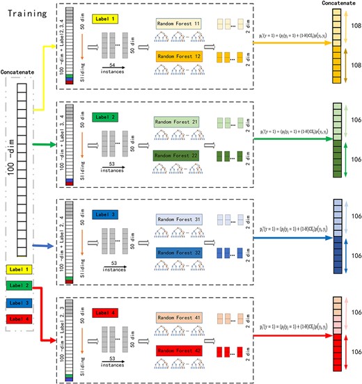
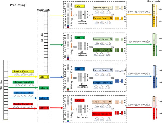
(A) Illustration of multi-grained scanning in training. Suppose there are four labels, raw features are 100-dim, and sliding window is 50-dim in the training of the first label. (B) Illustration of multi-grained scanning in predicting. Suppose there are four labels, raw features are 100-dim, and sliding window is 50-dim in the predicting of the first label.
Continued.
As shown in Figure 1B, in the prediction phase, probability is predicted first with traditional random forest for each label and concatenated to raw features. Probability of each label in the test data is predicted in the sequence of concurrence. Label with low concurrence rate is trained first.
Cascade forest
In the layer-wise cascade forest, the powerful classifier, random forest, is ensembled in each layer. In the classification to each label, the feature importance is considered assuming that the discriminative features should take higher weights. In the most correlated labels, this discriminative feature may also contribute to the classification of other labels. Boost class distribution vectors are generated by two random forests (one for complete random forest, the other for partial random forest) for both multi-grained scanning and cascade forest periods. The performance of each layer is evaluated with k-fold cross-validation [35, 36] to overcome the risk of overfitting. And in the cascade forest, the propagation will be terminated when there is no significant improvement to the performance of the whole cascade on validation set.
Overall procedure of MLCDForest
As the gcForest, there are two main components in the framework of MLCDForest. In the multi-grained scanning part, the corresponding transformed feature representation is classified according to different forests. And in the cascade forest, layer-wise random forest is to get more discriminative representations. The example of MLCDForest is illustrated for the first label in Figure 2. Two window sizes (50, 80) are used in multi-grained scanning for the data with 100 dimensions. |$(54+53+53+53)\times 2\times 2$| and |$(24+23+23+23)\times 2\times 2$| dimensional feature vectors are obtained for the window size of 50 and 80,respectively. Combining these feature vectors to different labels together with the correlation statistics, a 1224-dimensional transformed feature vector is available here if there are only four labels. In the cascade forest, the cascade-wise random forest is learnt with such 1224-dimensional feature vector, and the process will be terminated when the performance of the validation set is not significantly improved.
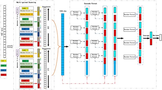
Overall procedure of MLCDForest. Suppose there are two classes, raw features are 100-dim, and sliding windows are 50-dim and 80-dim.
In any test instance, a 1224-dimensional representation vector, generated with multi-grained scanning, is the input data to the cascade forest to get its final prediction to each label by taking its class according to the maximum aggregated value.
Performance measures
Performance of different methods in multi-label classification is evaluated from the example-based, label-based and ranking-based [31]. In order to evaluate the generalization ability of MLCDForest, we utilized cross-validation in this study.
Example-based performance evaluation
Label-based performance evaluation
Ranking-based performance evaluation
Experiments and results
To evaluate the effectiveness of our proposed method, MLCDForest was compared with other multi-label classification methods: Deep Back-Propagation Neural Network (DBPNN) [38,39], RAkEL [22], MLkNN, BR and BPMLL [20] over this lncRNA dataset [40].
Datasets and hyperparameters
Data to associations between specific disease and lncRNAs [40] was employed in the construction of the proposed method. In the data downloaded from http://biomecis.uta.edu/∼ashis/res/csps2014/suppl/, 7566 lncRNA transcripts with 22 tissue labels were selected from the Human Body Map Project [41] with annotation and expression information of these 21,626 distinct lncRNAs. Eighty-nine composition-based features and 21 secondary structure-based features were identified with tissue-specificity threshold and as the input feature for different tissue classification. The detail information can be checked in [40].
In the experiments the division of the data in training and test set, which follows stratified approach [42], is in ratio of 80% versus 20%. Multi-grained scanning was based on 500 trees in each forest, and there were 1000 trees in the cascade forest as the default. In both multi-grained scanning and cascade forest, two completely random forests and two partial random forests were used in the training and prediction. In the two partial random forests, |$\sqrt{d}$| of features were selected as the candidates and separated with gini values. Fivefold cross-validation is used to evaluate the overall accuracy to overcome over-fitting. Comparing MLCDForest with DBPNN, which is conducted with Meka [39] and set the base classifier as random forest, other hyperparameters are the same as recommended in Meka. In [40], BR and RAkEL are based on sequential minimal optimization with support vector machines (SVMs) as base classifier. The number of nearest neighbors is 10 in MLkNN. And 10-fold cross-validation was conducted.
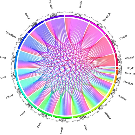
One major advantage of multi-label learning framework is to explore label correlations. Bias-corrected Cramér’s V statistics was calculated for all the label in label pairs and depicted them in a heat map (Figure 3A). Label concurrence is depicted in Figure 3B and Supplementary Table S1. Twenty out of 22 tissues are with standard CV of |$\mathrm{SCUMBLE}<0.8$|, 14 tissues are with standard CV of |$\mathrm{SCUMBLE}<0.75$|, and 8 tissues are with standard CV of |$\mathrm{SCUMBLE}<0.7$|. Tissues Foreskin_R and LF_r2 take the standard CV of 0.366 and 0.157 correspondingly. Details about the standard CV of |$\mathrm{SCUMBLE}$| can be found in Supplementary Table S1. Details about the pairwise corrected Cramér’s V statistics and pairwise intersections plot between all the labels are appended as Supplementary Table S2 and Supplementary Figure S1.
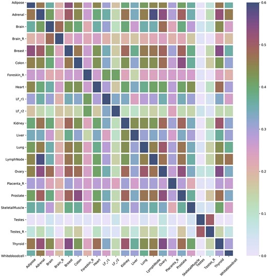
(A) Heat map of the correlation between tissues. (B) Concurrence to tissues based on SCUMBLE.
Continued.
Performance comparison
Performance comparison of the MLCDForest and other multi-label classifiers are presented in Tables 1–3. The MLCDForest achieved the best performance. In example-based evaluation from Table 1, it has achieved about 13% improvement in accuracy compared to MLkNN [40] and 16% in the precision compared to BR [40]. It is about 10% improvement in the label-based evaluation (Table 2) and similar performance in ranking-based evaluation (Table 3). As the performance of standard gcForest presented in [23] for single-label classification, neural network has shown to be better in the precision from example-based and label-based evaluation, but did not have similar performance from any evaluation aspect when compared to MLCDForest. This is because the dataset [40] is a small-scale biology data and deep neural network is highly dependent on the scale of dataset.
Label-wise evaluation
With the multi-label learning models, label-wise manner was also performed to check the performance for each label. Performance of MLCDForest can be checked in Table 4, which was conducted in 5-fold cross-validation.
Example-based evaluation of the predictive performance of different multi-label classifiers
| Hamming loss | Accuracy | Precision | Recall | F1-measure | Subset accuracy | |
|---|---|---|---|---|---|---|
| MLCDForest | 0.1145 | 0.6978 | 0.8402 | 0.7400 | 0. 6978 | 0.3347 |
| DBPNN | 0.2118 | 0.4811 | 0.8258 | 0.4999 | 0.5997 | 0.1636 |
| RAkEL [36] | 0.2032 | 0.5471 | 0.7781 | 0.6133 | 0.6409 | 0.1980 |
| MLkNN [36] | 0.1970 | 0.5610 | 0.7599 | 0.6486 | 0.6627 | 0.1807 |
| BR [36] | 0.2048 | 0.5441 | 0.7804 | 0.6050 | 0.6405 | 0. 1965 |
| BPMLL [36] | 0.2241 | 0.5191 | 0.6900 | 0.6660 | 0.6412 | 0.1006 |
Label-based evaluation of the predictive performance of different multi-label classifiers
| Micro-avg | Macro-avg | |||||
|---|---|---|---|---|---|---|
| Precision | Recall | F1 | Precision | Recall | F1 | |
| MLCDForest | 0.8603 | 0.7947 | 0.8262 | 0.8496 | 0.7170 | 0.7682 |
| DBPNN | 0.8556 | 0.4586 | 0.5971 | 0.7610 | 0.3160 | 0.3726 |
| RAkEL [36] | 0.7680 | 0.6219 | 0.6872 | 0.6625 | 0.4948 | 0.5494 |
| MLkNN [36] | 0.7698 | 0.6439 | 0.7011 | 0.6998 | 0.5237 | 0.5804 |
| BR [36] | 0.7766 | 0.6029 | 0.6788 | 0.5787 | 0.4588 | 0.5058 |
| BPMLL [36] | 0.7043 | 0.6497 | 0.6754 | 0.5753 | 0.4827 | 0.4700 |
Label-wise analysis of MLCDForest
| Tissue | Accuracy | Precision | Recall | F1 score | ROCAUC |
|---|---|---|---|---|---|
| Adipose | 0.8902 | 0.8788 | 0.7477 | 0.8080 | 0.8375 |
| Adrenal | 0.8936 | 0.9066 | 0.8573 | 0.8813 | 0.8845 |
| Brain | 0.8601 | 0.8555 | 0.8054 | 0.8297 | 0.7770 |
| Brain_R | 0.9393 | 0.9016 | 0.6445 | 0.7517 | 0.5561 |
| Breast | 0.8751 | 0.8303 | 0.8594 | 0.8446 | 0.8501 |
| Colon | 0.8705 | 0.8302 | 0.7483 | 0.7871 | 0.8236 |
| Foreskin_R | 0.9503 | 0.8205 | 0.4507 | 0.5818 | 0.7215 |
| Heart | 0.8902 | 0.8875 | 0.7058 | 0.7863 | 0.6596 |
| LF_r1 | 0.8994 | 0.8868 | 0.5465 | 0.6763 | 0.6556 |
| LF_r2 | 0.9740 | 0.7727 | 0.3208 | 0.4533 | 0.7186 |
| Kidney | 0.8480 | 0.8585 | 0.7665 | 0.8099 | 0.7995 |
| Liver | 0.8728 | 0.8062 | 0.5347 | 0.6430 | 0.5528 |
| Lung | 0.8231 | 0.7484 | 0.8223 | 0.7836 | 0.8439 |
| Lymph node | 0.8751 | 0.8318 | 0.8393 | 0.8356 | 0.9018 |
| Ovary | 0.8480 | 0.9048 | 0.7432 | 0.8160 | 0.7531 |
| Placenta_R | 0.9104 | 0.8095 | 0.5113 | 0.6267 | 0.7615 |
| Prostate | 0.8549 | 0.8327 | 0.8557 | 0.8441 | 0.8825 |
| Skeletal muscle | 0.8954 | 0.8320 | 0.6103 | 0.7041 | 0.6988 |
| Testes | 0.8936 | 0.8922 | 0.9944 | 0.9405 | 0.8336 |
| Testes_R | 0.9029 | 0.9288 | 0.9297 | 0.9292 | 0.9601 |
| Thyroid | 0.8699 | 0.8577 | 0.8420 | 0.8498 | 0.8661 |
| White blood cell | 0.8647 | 0.8187 | 0.6381 | 0.7172 | 0.7342 |
Discussion
As an alternative to deep learning, deep forest has been proven to be very powerful in the single-label classification in practice. However, most of practical biology classifications are multi-label classification problem. As one of the novel implementations and application of the standard deep forest model (gcForest), we emphasize the correlation and concurrence of labels in the data transformation. It is shown to be an effective method in the multi-label classification to lncRNA-disease associations. Our MLCDForest method provides an effective option to investigate multi-label classification by using deep learning on small-scale biology datasets.
Based on the data to associations between specific disease and lncRNAs [40], MLCDForest is compared with other multi-label classification approaches in the performance metrics. The proposed model has achieved the best performance on the dataset with original features. In the present study, we made an initial and rough attempt to incorporate the label correlation in sequential manner into the deep forest framework. In further study, we will test our proposed approach on more strictly experimental settings and apply it on more similar bioinformatics problems. Based on various types of association between ncRNAs, ncRNAs and disease, ncRNA and drug targets, small molecules and ncRNAs, genome analysis applications, etc. [43–48], we should perform further evaluation based on other independent dataset (i.e., association between miRNA–circRNA associations).
Predicting lncRNA-tissue association using computational methods is very important in disease diagnosis and therapy.
Label correlation is considered in multi-label classification with frame of MLCDForest
Funding
Dong-Qing Wei is supported by the grants from the Key Research Area Grant 2016YFA0501703 of the Ministry of Science and Technology of China, the National Natural Science Foundation of China (Contract no. 61832019, 61503244), the Science and Technology Commission of Shanghai Municipality (Grant: 19430750600), the Natural Science Foundation of Henan Province (162300410060) and Joint Research Funds for Medical and Engineering and Scientific Research at Shanghai Jiao Tong University (YG2017ZD14). The computations were partially performed at the Peng Cheng Lab and the Center for High-Performance Computing, Shanghai Jiao Tong University.
Wei Wang is a PhD student at the School of Mathematical Sciences, Shanghai Jiao Tong University. He works on statistical learning algorithm for the drug discovery.
Qiuying Dai is a PhD student at the School of Life Sciences and Biotechnology, Shanghai Jiao Tong University. She works on predicting circRNA-disease associations through machine learning methods.
Fang Li is a lecturer at the School of Life Sciences and Biotechnology, Shanghai Jiao Tong University. She works on drug discovery through machine learning methods and molecular simulation.
Yi Xiong is an associate professor at the School of Life Sciences and Biotechnology, Shanghai Jiao Tong University. His main research interests focus on machine learning algorithms and their applications in the protein sequence–structure–function relationship and biomedicine.
Dong-Qing Wei is a full professor at the School of Life Sciences and Biotechnology, Shanghai Jiao Tong University, State Key Laboratory of Microbial Metabolism and Joint Laboratory of International Cooperation in Metabolic and Developmental Sciences, Ministry of Education, Shanghai Jiao Tong University and Peng Cheng Laboratory, Vanke Cloud City Phase I Building 8, Xili Street, Nanshan District, Shenzhen, Guangdong. His main research areas include structural bioinformatics and biomedicine.
References
