


Abstract
Scoring functions (SFs) based on complex machine learning (ML) algorithms have gradually emerged as a promising alternative to overcome the weaknesses of classical SFs. However, extensive efforts have been devoted to the development of SFs based on new protein–ligand interaction representations and advanced alternative ML algorithms instead of the energy components obtained by the decomposition of existing SFs. Here, we propose a new method named energy auxiliary terms learning (EATL), in which the scoring components are extracted and used as the input for the development of three levels of ML SFs including EATL SFs, docking-EATL SFs and comprehensive SFs with ascending VS performance. The EATL approach not only outperforms classical SFs for the absolute performance (ROC) and initial enrichment (BEDROC) but also yields comparable performance compared with other advanced ML-based methods on the diverse subset of Directory of Useful Decoys: Enhanced (DUD-E). The test on the relatively unbiased actives as decoys (AD) dataset also proved the effectiveness of EATL. Furthermore, the idea of learning from SF components to yield improved screening power can also be extended to other docking programs and SFs available.
Introduction
As the most important approach used in structure-based virtual screening (SBVS), molecular docking can predict how a ligand binds to its biomolecular target and estimate the binding affinity between the ligand and target [1–3]. Operationally, the docking process consists of two basic stages: predicting the position, orientation and conformation of the ligand when docked into the binding pocket of a certain protein (pose generation or conformational sampling) and estimating how strongly the docked poses bind to the target (scoring). Correspondingly, the reliability of molecular docking depends on the coverage of pose generation and the accuracy of binding affinity predicted by scoring functions (SFs) [4, 5].
It must be recognized that SFs are created on the basis of some essential simplifications for the sake of efficiency [6, 7], which is the reason why no individual SFs could cover the whole process of protein–ligand recognition. However, SFs could still efficiently enrich active molecules from a huge pool of candidate compounds, and many successful applications have been publicly reported [8–12]. Actually, the state-of-the-art docking programs have worked reasonably well in conformation sampling, but the inaccuracies in the prediction of binding affinity by SFs continue to be the major limiting factor for more reliable docking, which is also one of the most important open problems in computational chemistry [13].
SFs can be roughly classified into two major categories from the view of methodology: classical SFs (i.e. force field, empirical, knowledge, etc.) and machine learning (ML)-based SFs [14]. Most SFs implemented in docking programs belong to classical SFs, for which a common characteristic is that they normally take the form of linear regression with a small number of expert-selected features (i.e. non-bonded interaction terms, solvent accessibility surface area (SASA), atom pairwise contacts, etc.), assuming there is a theory-motivated functional form for the relationship between the binding affinity and the features characterizing a complex even though the linear relationship may not exist at any time [15]. On the contrary, ML-based SFs prefer to learn from very large volumes of structural and interaction data instead of making linearity as their assumption [16]. Consequently, these ML-based SFs have the ability to capture nonlinear binding interactions that are difficult to be characterized by classical SFs, thus yielding better binding affinity predictions. ML-based SFs have seen a surge in popularity for their superiority over classical SFs. The past few years have witnessed significant advances in ML-based SFs, and the development of ML-based SFs can be envisaged along two aspects: exploring novel protein–ligand interaction characterization and switching to alternative ML algorithms. With respect to the characterization, knowledge-based pairwise potentials [17–20], terms extracted from existing SFs [21–23] and protein–ligand interaction-related descriptors/fingerprints[24, 25] are the most popular representation methods. Besides, a wide variety of ML algorithms, including random forest (RF) [16, 26, 27], support vector machine (SVM) [24, 28], artificial neural network (ANN) [29, 30], gradient boosting decision tree (GBDT) [31] and convolutional neural network (CNN) [32] have been used to build ML-based SFs.
For normal academic researchers, the commonly used docking programs, such as MOE [33], Glide [34, 35], GOLD [36], AutoDock [37] and AutoDock Vina [38], which have been developed and continually updated, are still their first choice when conducting VS considering the maneuverability and availability. Usually, the final score is the only criterion to decide if a ligand can bind to its target or not. However, rather than a total score of the docked ligand, SFs could provide many detailed energy auxiliary terms which can reflect the features of protein–ligand recognition to some extent. Taking Goldscore, one of the SFs employed in GOLD, as an example, Goldscore is able to supply additional energy terms for various types of interactions, such as protein–ligand H-bond, van der Waals, ligand torsion strain and other energy auxiliary terms along with the total score (Goldscore.Fitness). A straightforward question may be raised: can classical SFs be improved by optimizing their scoring components through ML algorithms?
Actually, some researchers have examined the potential benefit of the combination of the scoring components of existing SFs or interaction energy components and ML. For example, MIEC-GBDT was a VS classification model whose prediction accuracy achieved 87% for luciferase inhibitors [39]. Molecular interaction energy components (MIEC) were extracted from the decomposition of molecular mechanics/generalized born surface area (MM/GBSA), and then the GBDT algorithm was employed to build the MIEC-GBDT classification model. Yasuo et al. proposed a novel approach referred to as similarity of interaction energy vector score (SIEVE-Score) [40], which was trained by random forest based on the per-residue interaction energy terms extracted from the Glide-SP docking results. The SIEVE-Score showed much better performance than popular docking programs in distinguishing active compounds, but it also needed more known experimental data and expert interventions. Yunierkis et al. put forward CompScore [41] by simply incorporating the information provided by SF components into a consensus scoring scheme [42] to obtain boosted virtual screening (VS) performance without training any ML model. The above reported studies demonstrate that energy components may be effective features to represent protein–ligand recognition so that the existing popular docking programs and SFs are worth further exploration.
In this paper we presented a novel and handy approach based on the scoring components extracted from the output of the SFs implemented in several popular docking programs. The diverse subset of the Directory of Useful Decoys: Enhanced (DUD-E) [43] was used to test our approach. Each molecule in DUD-E was docked into its target using several popular docking programs. Then different levels of ML models were built based on the scoring components yielded in the last stage, and the major focus in the evaluation should be paid to the screening power, the capability to identify actives from decoys. Through this study, we expect to gain more insight into the following three questions. (i) Here, advanced ML algorithms were employed to develop improved SFs including EATL SFs, docking-EATL SFs and comprehensive SFs by analyzing different combinations of scoring components given by multiple classical SFs. Therefore, can the screening power of our improved SFs be improved compared with that of the classical SFs? (ii) Many ML-based SFs have proved themselves in the field of VS, so can our model achieve comparable results to other advanced SFs or methods? (iii) It is reported that the DUD-E benchmark may suffer from negative bias resulting from the decoys selection criteria, rendering the actives more distinguishable from the decoys. Accordingly, can our proposed method still yield a satisfactory performance on another relatively unbiased dataset?
Materials and methods
Validation dataset
The diverse subset of the DUD-E dataset [43], broadly accepted for benchmarking VS protocols, was used to test our approach. The whole DUD-E dataset consists of 102 target proteins, and the diverse subset of DUE-E contains 8 target proteins belonging to seven broad protein categories. Hence, the diverse subset is qualified to stand for the whole DUD-E dataset to some extent. More information about the subset is shown in Table 1. The active and inactive compounds for each target were taken from the ChEMBL [44] and ZINC [45] databases, respectively. The ratio of actives to inactives (decoys) for each target is 33.1 on average. Structurally similar active compounds have already been filtered out by clustering analysis. The decoys were chosen to resemble ligands physically in order to fulfill their role as negative controls which were challenging for docking but topologically dissimilar to minimize the likelihood of actual actives. Generally, there are no identical or excessively similar data for each target. The DUD-E benchmark is available at http://dude.docking.org/
Information of the diverse subset of DUD-E
| Target | PDB | Description | Class | Actives | Decoys |
|---|---|---|---|---|---|
| AMPC | 1l2s | Beta-lactamase | Other enzymes | 62 | 2902 |
| CXCR4 | 3odu | C-X-C chemokine | GPCR | 122 | 3414 |
| KIF11 | 3cjo | C-X-C chemokine receptor type 4 | Miscellaneous | 197 | 6912 |
| CP3A4 | 3nxu | Cytochrome P450 3A4 | CYP450 | 363 | 11 940 |
| GCR | 3bqd | Glucocorticoid receptor | Nuclear | 563 | 15 185 |
| AKT1 | 3cqw | Serine/threonine–protein kinase Akt-1 | Kinase | 423 | 16 576 |
| HIVRT | 3lan | HIV type 1 reverse transcriptase | Other enzymes | 639 | 19 134 |
| HIVPR | 1xl2 | HIV type 1 protease | Protease | 1395 | 36 278 |
The actives as decoys (AD) dataset, a relatively unbiased version of DUD-E, was recently proposed by Kurtzman et al. in their work investigating the impact of potential biases in DUD-E on the performance of CNN models [46]. The AD dataset consists of the same 102 targets and inherits the active datasets of DUD-E, while its decoy sets are entirely differen. For each target in the AD dataset, all the actives from other 101 targets were docked to the identified protein target by Vina, one after another. Then the top 50 actives of the 101 targets ranked by binding affinity (approximately 5050, 50 × 101) were selected to comprise the decoy set for the docked target. Due to the special decoy selection criteria, it seems that the AD dataset is a more challenging VS benchmark for scoring evaluation schemes. Here we chose the same eight targets as the diverse subset for further strategy validation. The complete constructed AD dataset for 102 targets is freely available at www.lehman.edu/faculty/tkurtzman/files/102_targets_AD_dataset.tar
Protein–ligand docking and rescoring
All the eight targets from the diverse subset were utilized for the validation of our methodology. Compounds were preprocessed by OMEGA [47] to yield appropriate conformations and isomers. Proteins were processed by the protein preparation and energy minimization module implemented in MOE (version2018.01). During the docking calculations with MOE, the binding site was defined by the co-crystalized ligand included in the DUD-E file, and the conformation search of each molecule was conducted with the triangle matcher algorithm. Each compound contains 30 docking poses after conformational sample, and only the top-scored one was kept for the following rescoring.
The top-scored poses were then rescored with MOE dock (version2018.01), GOLD (version5.3.0), and Schrodinger Glide (version7.1), respectively, with all default parameters unless otherwise specified. All the SFs implemented in MOE and GOLD were employed for rescoring, whereas for Glide only the standard precision (SP) mode was employed considering the efficiency and precision.
Scoring functions and components
The features used for model training are the scoring components extracted from the rescoring output files. The basic information of the 10 SFs and the corresponding scoring components is summarized in Table 2, and additional descriptions can be found in Supplementary Table S1. Of note, all the scoring components are energy terms representing the protein–ligand recognition instead of only ligand-based features which are not sufficient for prediction of binding possibility due to the lack of information about the receptor. Here we defined these scoring functions components as energy auxiliary terms (EATs).
Information of the SFs and scoring components of each docking program
| Software | SF | Scoring components | Number of components |
|---|---|---|---|
| MOE (version2018.01) | Affinity-dG | S, E_conf, E_score1, E_refine E_place | 5 |
| Alpha-HB | S, E_conf, E_score1, E_refine, E_place | 5 | |
| GBVIWSA-dG | S, E_conf, E_score1, E_refine, E_place | 5 | |
| London-dG | S, E_conf, E_score1, E_refine, E_place | 5 | |
| ASE | S, E_conf, E_score1, E_refine, E_place | 5 | |
| GOLD (version5.3.0) | Goldscore | Goldscore.Fitness, Goldscore.External.HBond Goldscore.External.Vdw Goldscore.Internal.Torsion Goldscore.Internal.Vdw | 5 |
| ChemPLP | PLP.Fitness,PLP.PLP, PLP.Chemscore.Hbond,PLP.ligand.torsion, PLP.part.buried,PLP.part.hbond, PLP.part.nonpolar, PLP.part.repulsive | 8 | |
| ASP | ASP.Fitness, ASP.ASP, ASP.DEClash, ASP.DEInternal, ASP.Map | 5 | |
| Chemscore | Chemscore.Fitness, Chemscore.DEClash, Chemscore.DEInternal, Chemscore.DG, Chemscore.Hbond, Chemscore.Lipo, Chemscore.Rot | 7 | |
| Schrödinger (version7.1) | GlideScore-SP | docking score, glide ligand efficiency, glide ligand efficiency sa, glide ligand efficiency ln, glide gscore, glide lipo, glide hbond, glide rewards, glide evdw, glide ecoul, glide erotb, glide esite, glide emodel, glide energy, glide einternal | 15 |
Model training
Five-fold cross-validation (CV) [48] was employed to evaluate the performance of the derived models. In practice, the data are first partitioned into five equally sized segments. Subsequently five iterations of training and validation were performed such that 4-folds of the data were utilized for learning and the remaining 1-fold was used for validation within each iteration. In addition, stratified CV [49] was used to ensure that the class distribution is kept as close as possible to be the same across all folds. As mentioned above, our dataset is unbalanced (the ratio of the decoys versus actives is approximately 33 on average), so the undersampling strategy was conducted on the negative samples to make its number the same as that of the positive samples for each segment in the training set; in other words, the final training set consists of the same numbers of actives and decoys [50]. On the purpose of fully utilizing the negative data, the undersampling process was repeated 100 times.
Extreme gradient boosting (XGBoost) [51], a type of gradient boosting decision tree method, was used to construct the classification model. The XGBoost model has been widely used in all kinds of data mining fields [52–54] as well as the development of ML-based SFs [55, 56]. Both the first and second derivatives of the loss function are used, which enables the algorithm to coverage the global optimality faster and improve the efficiency of the optimal solution of the model. The main hyper-parameters of XGBoost, including the learning rate, the maximum depth of a tree and the boosting rounds, were optimized by the grid search method and 5-fold cross-validation. In our study, the output of a XGBoost classifier is the predicted possibilities of true binders in a scale of 0∼1. The final prediction of each compound is the arithmetic mean of the 100 predictions. All the models were implemented in KNIME (version3.7.1) [57]. In addition, the input feature files and workflow can be downloaded here ( https://github.com/xiongguoli/data_EATs-learning ).
Evaluation metrics
To rigorously evaluate the performance of our model, the enrichment factor (EF) values at the 0.1%, 0.5%, 1%, 2% and 5% levels, the area under the curve (AUC) of receiver operating characteristic (ROC) curve, the Boltzmann-enhanced discrimination of receiver operating characteristic (BEDROC) score and log-scaled area under the receiver-operating characteristic curve (LogAUC) were adopted in the screening power assessment. All the metrics were calculated by in-house Python scripts.
The EF values are commonly used in VS evaluation as accuracy metrics. The EFx% value is defined as the ratio between the predicted hit rate and the random hit rate when the top x% ranked compounds are selected as actives. The ROC curve reflects the relationship between the sensitivity and specificity [58]. The AUC is defined as the area under the ROC curve to measure the overall performance of docking enrichment. The possible values of the AUC range from 0 to 1 and the AUC values corresponding to ideal and random prediction are 1 and 0.5, respectively. In simple words, the larger the AUC value, the better the model performs. The BEDROC score is generalized to incorporate a weighting function that adapts it for use in early recognition problems. For each protein, the BEDROC score takes all the compounds into account rather than being limited to a percentile of the chemical library as EFX%. Simultaneously, the score can be modulated by the weight given to the top-ranked compounds by adjusting the parameter α. In this study, the parameter α was set to 80.5, which means the 2% top-ranked molecules account for 80% of the BEDROC score [59]. LogAUC was introduced to tackle the early enrichment problem by computing the percentage of the ideal area that lay under the semilog ROC curve. Formally, we defined LogAUCλ, where the log area was computed from λ = 0 to 1.0, and in this study LogAUC0.001 was simply denoted by LogAUCλ [60].
Results and discussion
The performance of EATL SFs
We constructed the EATs learning (EATL) SFs for each target by employing the EATs provided by each classical SF as the input features for training. The ROC curves and associated AUCs of each classical and EATL SFs are illustrated in Figure 1. Comparison between the classical and EATL SFs in terms of the AUC-ROC values and BEDROC scores are shown in Figures 2 and 3. The detailed results obtained for the diverse subset are provided as Supplementary Table S2.
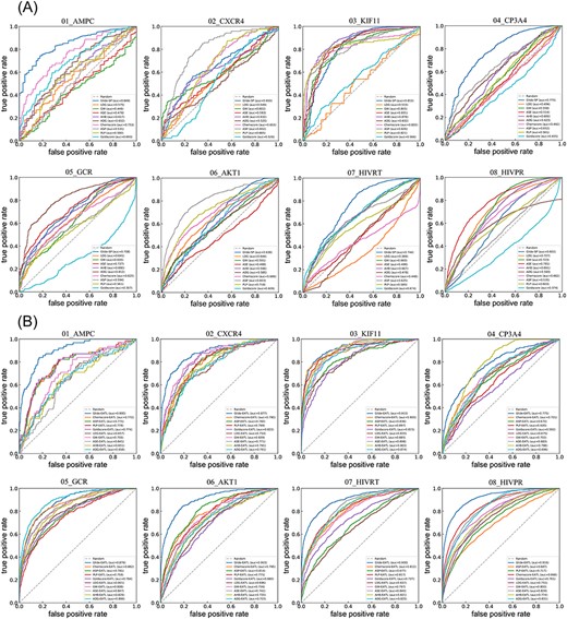
ROC curves of 10 classical SFs (A) and EATL SFs (B) on 8 targets. ADG, affinity dG; AHB, alpha HB; ASE, ASE; GW, GBVI/WSA dG; and LDG, London dG. And the dashed line indicates random selection.
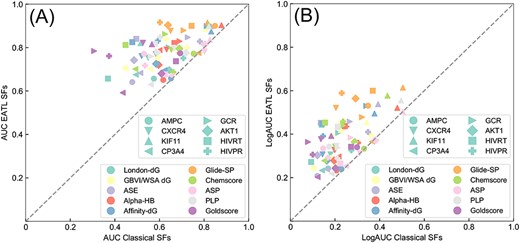
Scatter plots of the AUC-ROC (A) and LogAUC (B) results of classical and EATL SFs. The shape and color of each point represent the target and SF, respectively. And the dashed line indicates the limit where both scoring schemes perform equally.

Box plot of the BEDROC (α = 80.5) results of classical and EATL-SFs. The horizontal lines indicate median, and the plus signs represent the mean BEDROC score. ADG, affinity dG; AHB, alpha HB; ASE, ASE; GW, GBVI/WSA dG; and LDG, London dG. The plot is built with the values of BEDROC for all the targets as provided in Supplementary Table S2.
It can be seen from Figure 1A that some classical SFs can yield satisfactory performance on some targets such as Glide-SP for AMPC (0.849), Alpha-HB for KIF11 (0.878) and Affinity-dG for GCR (0.812) but perform badly on other targets whose values are even lower than a random level (0.5) such as Goldscore for GCR (0.307), London-dG for HIVRT (0.369) and Goldscore for HIVPR (0.374), even though the improvement over the random level is statistically significant (P < 0.05) across the dataset for most classical SFs except for London-dG and Goldscore. Among all the 10 classical SFs, Glide-SP can achieve the best performance (0.723) on average. However, the SFs from MOE and GOLD can only obtain the values ranging from 0.523 to 0.671 on average, implying that it’s hard for most classical SFs to distinguish ligands from decoys in VS campaigns. While for our EATL SFs (Figure 1B), each of the AUC values is far higher than 0.5, with 34 of them reaching the AUC values above 0.8. In addition, some EATL SFs can yield remarkable performance on certain targets, such as Glide-EATL for KIF11 (0.915) and HIVPR (0.916). The comparison results for LogAUC are similar to those for AUC, as shown in Supplementary Figure S1.
For comparison, Figure 2 presents the scatter plot of the ROC-AUC (A) and LogAUC (B) results for classical SFs versus EATL SFs. The shape and color of each point represent the target and SF, respectively. Our EATL SFs achieve improved VS performance by considering the two metrics for all the scoring schemes across the dataset, and the improvement is statistically significant (P = 3.4 × 10⁻¹⁷ and 3.4 × 10⁻¹⁴ for ROC-AUC and LogAUC, respectively) in the light of the paired t-test. Further learning of the SF components renders the AUC to grow at an astonishing average of 24.67%. More importantly, it is interesting to observe that the worst mean AUC values provided by the EATL SFs are even higher than the best value provided by the classical SFs.
Next, BEDROC with α = 80.5 (see Materials and methods) was chosen to work out the ‘early recognition’ problem and to weight the contribution of the rank axis to the final score. As illustrated in Figure 3, sharp differences exist among the classical SFs implemented in different docking programs. Glide-SP can still yield the best performance in terms of the early recognition ability. The worst early enrichment is obtained when employing London-dG, and most other classical SFs have similar poor performance (lower than 0.2). Based on the mean BERROC values, the early recognition power of classical SFs has the following rank: Glide-SP (0.274) > ASP (0.196) > Alpha-HB (0.173) > PLP (0.156) > Chemscore (0.145) > GBVI/WSA-dG (0.133) > ASE (0.113) > Goldscore (0.085) > Affinity-dG (0.083) > London-dG (0.060). Similar to the results shown in the previous section, further learning of the SF components using XGBoost (in blue) leads to the obvious improvement of the BEDROC scores relative to classical SFs (in red). This supports our hypothesis that the SF components could provide meaningful information on protein–ligand interactions and learning from these energy auxiliary terms using ML algorithms could compensate the weaknesses of individual scoring terms to better serve VS campaigns.
The performance of docking-EATL SFs
After comparing classical and EATL SFs, our new feature-based learning method has demonstrated the huge superiority in screening power. Hence, we also explored whether the learning of all the energy auxiliary terms from the same docking program defined as docking-EATL SFs could outperform the previous EATL SFs. The ROC and semilog ROC curves of the docking-EATL SFs and the best-performed EATL SF for each docking program (ASE for MOE and Chemscore for GOLD) are illustrated in Figures 4 and 5. The results of EF are presented as Supplementary Table S3, and the distributions of EF across targets are shown in Figure 6. The BEDROC scores of the tested models are listed in Table 3.
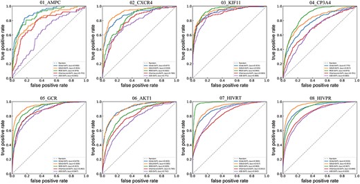
ROC curves of docking-EATL SFs and the best EATL SFs across the eight targets. Chemscore-EATL and ASE-EATL are the best EATLs SF of GOLD and MOE, respectively. And the dashed line indicates random selection.
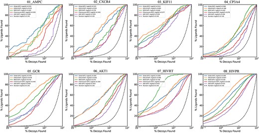
Semilog ROC curves of docking-EATL SFs and the best EATL SFs across the eight targets. Chemscore-EATL and ASE-EATL are the best EATLs SF of GOLD and MOE, respectively. And the dashed line indicates random selection.
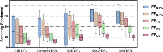
EFs at the top 0.1%, 0.5%, 1%, 2% and 5% levels distributions of docking-EATL SFs and the best EATL SFs across the eight targets. The horizontal lines indicate median, and the plus signs represent the mean enrichment factor. The plot is built with the values of EF at different levels for the eight targets as provided in Supplementary Table S3.
Comparison of BEDROC values for docking-EATL and the best EATL SFs on eight targets
| Target | ASE-EATL | Chemscore-EATL | MOE-EATL | GOLD-EATL | Glide-EATL |
|---|---|---|---|---|---|
| AMPC | 0.056 | 0.196 | 0.294 | 0.371 | 0.504 |
| CXCR4 | 0.246 | 0.280 | 0.290 | 0.591 | 0.578 |
| KIF11 | 0.567 | 0.611 | 0.712 | 0.761 | 0.671 |
| CP3A4 | 0.085 | 0.166 | 0.277 | 0.338 | 0.324 |
| GCR | 0.444 | 0.341 | 0.604 | 0.737 | 0.442 |
| AKT1 | 0.158 | 0.241 | 0.208 | 0.532 | 0.552 |
| HIVRT | 0.518 | 0.546 | 0.778 | 0.670 | 0.711 |
| HIVPR | 0.440 | 0.537 | 0.597 | 0.772 | 0.710 |
| Mean | 0.314 | 0.365 | 0.470 | 0.597 | 0.562 |
| Median | 0.343 | 0.311 | 0.446 | 0.631 | 0.565 |
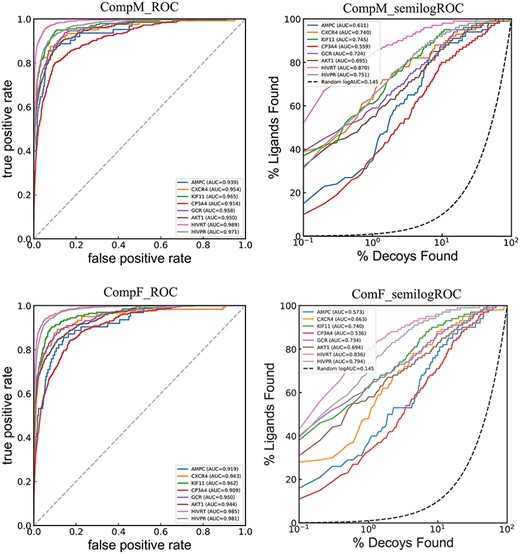
ROC and semilog ROC curves of CompF and CompM across the dataset.
A detailed analysis of the data presented in Figures 4 and 5 shows that the results of ROC-AUC and LogAUC share highly similar trends. For the sake of simplicity, our discussions will be mainly focused on ROC-AUC. Here, MOE-EATL and GOLD-EATL, trained with all the energy auxiliary terms provided by each docking program, can obtain eye-catching AUC performance, which exceeds the corresponding best EATL SFs (ASE-EATL and Chemscore-EATL, respectively) by 15.4% and 14.7% on average. The absolute ROC-AUC on AMPC can be improved from 0.641 to 0.876 by learning all the scoring components within MOE rather than those within ASE. Similarly, an improvement over 0.2 (from 0.687 to 0.953) can be observed on the target HIVPR by learning all the scoring components within GOLD instead of those within Chemscore. According to the averaged AUCs, an order of the docking-EATL SFs can be obtained: GOLD-EATL (0.901) > MOE-EATL (0.895) > Glide-EATL (0.883). While when the medians are regarded as the criteria, the order should be changed to GOLD-EATL (0.918) > Glide-EATL (0.900) > MOE-EATL (0.892). It should be noted that Glide, the docking module of Schrödinger, is different from the other tested docking programs with many SFs available to be chosen. Considering the precision and computation time, only the standard precision (SP) mode was selected for scoring. The SF under this mode is unique, and the number of the scoring components used for model training is far fewer than those of GOLD-EATL and MOE-EATL. However, the performance of Glide-EATL is definitely not inferior to its counterparts, indicating the 15 components from the Glide-SP docking mode are capable of capturing sufficient effective protein–ligand binding information to distinguish true ligands from decoys.
We also evaluated the performance of the docking-EATL SFs with respect to BEDROC. Similar to the previous findings, the docking-EATL SFs also outperform the corresponding top-ranked EATL SFs, and the improvement of BEDROC is statistically significant (P = 0.08 and 0.009 for MOE and GOLD, respectively). In addition, the improvements on the BEDROC scores by learning more scoring components can reach up to 49.6% and 63.5% for MOE and GOLD on average, respectively, which are quite higher than those on AUC. The largest improvement of the BEDROC score is observed for the AMPC target with 425% (over 5 times) from ASE-EATL (0.056) to MOE-EATL (0.294). We also find that the classical ASE SF achieves a BEDROC of 0.001 on this target, indicating that ASE may have some inherent defects on this target so that the components provided by ASE may be unable to characterize protein–ligand interaction patterns properly. However, our EATL method could compensate for the inherent defects of classical SFs to provide acceptable performance on both the SF and docking program levels. Overall, the rank of the docking-EATL SFs should be GOLD-EATL > Glide-EATL > MOE-EATL considering the mean and median BEDROC scores.
The distributions of the enrichment factors across the targets are shown in Figure 6. By closely examining EF at the top 0.1%, 0.5%, 1%, 2% and 5% levels (Supplementary Table S3), it can be found that the docking-EATL SFs have absolute superiority over EATL SFs in terms of initial enrichment. Apparently, GOLD-EATL and Glide-EATL are more suitable for VS campaigns due to their stable fluctuation ranges and larger medians, suggesting they are able to provide generally excellent initial enrichment on almost all kinds of proteins. One can also see from Figure 6 that MOE-EATL SF fails to generate excellent enrichment as good as the other two docking-EATL SFs and even has similar performance as the two EATL SFs although it yields acceptable results in terms of mean ROC-AUC. In truth, the enrichment factors should be more reliable metric because we usually pay more attention to top-ranked molecules after ranking large chemical database from the highest to lowest probabilities of binding to a certain target.
A closer look at the results in term of all the evaluation metrics shows that all the EATL SFs discussed in this section yield slightly worse performance on the targets CP3A4 and AMPC. We also checked the data of the other scoring schemes mentioned above, and the same phenomenon could be observed in most scoring schemes. The inherent characteristic of protein may contribute to the poor VS performance on the target CP3A4. CP3A4 is a major drug-metabolizing enzyme, which plays an important role in the metabolism of approximately 30% of clinical used drugs [61, 62]. Its binding pocket is rather wider and more flexible than most other proteins, ranging in volume from 950 Å3 to 2000 Å3 in the absence and presence of bound ligands [63, 64] so that diverse substrates and inhibitors can be accommodated in the active site, making scoring a difficult task. Therefore, it is not strange that learning popular SF components on CP3A4 could not obtain results as good as on the other targets. As for AMPC, the loss in accuracy may be explained by the bias in the training data. We know that this library constitutes only 62 ligands and four-fifth of the actives are available in the training set. Accordingly, the XGBoost model may not be able to distinguish active from decoys and give true binders higher prediction values by learning limited information.
Another interesting finding is that the impact of the target on the same scoring scheme is significant; in other words, no scoring schemes here can obtain good AUC values for all the eight targets simultaneously. Taking GOLD-EATL that has the most comprehensive excellent performance as an example, the BEDROC scores range from 0.371 (AMPC) to 0.772 (HIVPR). The same phenomenon is identified by the other scoring schemes and evaluation metrics. From this result, it’s pivotal to make a detailed scoring scheme assessment before VS campaigns to guarantee that the SFs used for docking is reliable. Future research efforts should be devoted to the development of target-customized SFs.
The performance of comprehensive EATL SFs
We also compared the predicted compounds given by the three docking-EATL SFs. Taking the target HIVPR as an example, the top 1% predicted compounds (343 compounds) were extracted from the three docking-EATL SFs for further analysis. A total of 238, 303 and 288 actives were identified by MOE-EATL, GOLD-EATL and Glide-EATL, respectively, in the top 1% lists. As to these actives, only 63 compounds could be identified by the three docking-EATL SFs simultaneously, 164 could be identified by two docking-EATL SFs, and 312 could be identified by a single docking-EATL SF. The results for the other targets are shown in Supplementary Figure S2. These findings indicate that the overlaps among the predictions given by the three docking-EATL SFs are not quite high, and therefore, there is a possibility to improve VS performance when these methods are appropriately combined.
To further explore whether the combination of these three docking-EATL SFs can provide boosting VS performance, two new experiments were performed. Firstly, all the 61 energy auxiliary terms extracted from the three docking programs were used as the input features to train a new comprehensive model named as CompF. The details about the model training are the same as the other EATL SFs mentioned above. The second experiment is based on the prediction results of the three docking-EATL SFs. For each compound in the library, the arithmetic mean of the predictions given by the three docking-EATL SFs was defined as the final prediction of each compound. We named this scoring scheme as CompM. The ROC and semilog ROC curves of the two comprehensive EATL SFs are shown in Figure 7. And the initial enrichment results are summarized in Table 4.
The VS performance of CompF and CompM
| Target | AUC | BEDROC | LogAUC | EF0.1% | ||||
|---|---|---|---|---|---|---|---|---|
| CompF | CompM | CompF | CompM | CompF | CompM | CompF | CompM | |
| AMPC | 0.919 | 0.939 | 0.545 | 0.574 | 0.573 | 0.611 | 32.258 | 32.258 |
| CXCR4 | 0.943 | 0.954 | 0.745 | 0.852 | 0.663 | 0.740 | 25.000 | 25.000 |
| KIF11 | 0.962 | 0.965 | 0.813 | 0.814 | 0.740 | 0.745 | 35.533 | 35.533 |
| CP3A4 | 0.909 | 0.914 | 0.540 | 0.574 | 0.536 | 0.559 | 19.608 | 33.613 |
| GCR | 0.950 | 0.958 | 0.807 | 0.784 | 0.734 | 0.724 | 37.143 | 37.143 |
| AKT1 | 0.944 | 0.950 | 0.727 | 0.713 | 0.694 | 0.695 | 44.248 | 44.248 |
| HIVRT | 0.985 | 0.989 | 0.906 | 0.931 | 0.836 | 0.870 | 30.201 | 30.201 |
| HIVPR | 0.981 | 0.971 | 0.895 | 0.862 | 0.802 | 0.751 | 24.229 | 24.963 |
Comparison with several other methods in terms of EF0.1% and BEDROC (α = 80.5)
| EF0.1% | GOLD-EATL | Glide-EATL | CompF | CompM | CompScore | CNN | DenseFS | SIEVE-Score | RF-Score-VS v3 |
|---|---|---|---|---|---|---|---|---|---|
| AMPC | 25.806 | 35.484 | 32.258 | 32.258 | 39.570 | 2.083 | 14.583 | 30.700 | 32.265 |
| CXCR4 | 20.000 | 20.833 | 25.000 | 25.000 | 51.610 | 5.000 | 5.000 | 61.100 | 60.853 |
| KIF11 | 33.503 | 30.457 | 35.533 | 35.533 | 51.340 | 11.207 | 4.310 | 53.400 | 4.527 |
| CP3A4 | 17.927 | 15.126 | 19.608 | 33.613 | 14.040 | 28.743 | 44.311 | 6.700 | 25.865 |
| GCR | 34.571 | 24.000 | 37.143 | 37.143 | 27.090 | 12.791 | 20.930 | 33.300 | 32.450 |
| AKT1 | 29.204 | 31.563 | 44.248 | 44.248 | 37.570 | 84.642 | 89.420 | 42.100 | 41.893 |
| HIVRT | 28.691 | 29.027 | 30.201 | 30.201 | 21.770 | 12.195 | 12.760 | 39.800 | 39.813 |
| HIVPR | 23.421 | 21.953 | 24.229 | 24.963 | 18.200 | 9.851 | 8.396 | 38.300 | 65.735 |
| BEDROC | GOLD-EATL | Glide-EATL | CompF | CompM | CompScore | GOLD | Glide | Surflex | Flex X |
| AMPC | 0.294 | 0.371 | 0.545 | 0.574 | 0.66 | 0.04 | 0.09 | 0.00 | 0.04 |
| CXCR4 | 0.290 | 0.591 | 0.745 | 0.852 | 0.71 | 0.08 | 0.01 | 0.27 | 0.01 |
| KIF11 | 0.712 | 0.761 | 0.813 | 0.814 | 0.84 | 0.55 | 0.59 | 0.12 | 0.08 |
| CP3A4 | 0.277 | 0.338 | 0.54 | 0.574 | 0.71 | 0.21 | 0.17 | 0.13 | 0.08 |
| GCR | 0.604 | 0.737 | 0.807 | 0.784 | 0.48 | 0.13 | 0.21 | 0.30 | 0.18 |
| AKT1 | 0.208 | 0.532 | 0.727 | 0.713 | 0.68 | 0.42 | 0.24 | 0.05 | 0.11 |
| HIVRT | 0.778 | 0.670 | 0.906 | 0.931 | 0.43 | 0.42 | 0.37 | 0.13 | 0.19 |
| HIVPR | 0.597 | 0.772 | 0.895 | 0.862 | 0.30 | 0.30 | 0.14 | 0.10 | 0.05 |
From Figure 7 and Table 4, it can be observed that CompF and CompM yield similar outstanding results with absolute predominance across the targets relative to a single EATL scoring scheme. Despite some improvements for CompM compared with CompF in terms of ROC-AUC, BEDROC, LogAUC and EF1%, the Wilcoxon matched-pairs signed rank test indicates the improvements are not statistically significant for all the four metrics. It should be noted that the performance achieved by CompF and CompM can be mainly attributed to the learning of these SF components with XGboost instead of a simple consensus scoring. The EF data in Table 4 and Supplementary Table S3 show that neither CompM nor CompF could bring about a big boost for the initial enrichment at the 0.1% level although the two comprehensive EATL SFs are indeed better VS scoring schemes. However, the comprehensive EATL models show better performance at the top 0.5% and 1% levels as provided in Supplementary Table S3.
Comparison with other methods
As MOE-EATL SF does not perform so well in the assessments of screening power, it was excluded from the comparison with other methods with relatively gratifying accuracy to the same dataset. Ragoza et al. proposed a convolutional neural network (CNN) SF that automatically learned the key features of protein–ligand interactions [65]. Then, based on previous work, Imrie et al. presented a deep learning approach named DenseFS that gives substantial improvement over the baseline CNN of Ragoza et al. in VS on DUD-E [66]. Besides, Yasuo et al. developed a new VS method named similarity of interaction energy vector score (SIEVE-Score), in which the van der Waals, Coulomb and hydrogen bonding interactions were extracted to represent docking poses for ML [40]. In the same work, RF-Score-VS v3, a state-of-the-art ML-based SF was evaluated as a comparison. Recently, Yunierkis et al. implemented and tested a new method named CompScore that used genetic algorithms to find the best combination of scoring components [41]. The comparisons between EATL and several other scoring schemes were conducted and the corresponding EF0.1%, and BEDROC are listed in Table 5. Note that the data for GOLD, Glide, Surflex and Flex X was from [67].
Firstly, consistent with previous findings, the initial enrichment performance of some models especially CNN and DenseFS is largely determined by the target library used for testing. For example, CNN can yield satisfactory enrichment factor on AKT1 (84.642) while poor enrichment on AMPC (2.083) relative to other scoring schemes. DenseFS and CNN both use direct and comprehensive 3D descriptions of complex structures as the input, implying that structure-based features may provide enough information on certain targets but fail to capture adequate information on others. From the color of each cell, we may conclude that SIEVE-Score and RF-Score-VS v3 should be the most applicable scoring schemes for the dataset despite the existence of extreme low values. However, it can be observed that the superiority of SIEVE-Score and RF-Score-VS v3 over our two comprehensive EATL SFs is not statistically significant according to the Wilcoxon matched-pairs signed rank test (95% confidence interval). Furthermore, CompF and CompM show absolute predominance in terms of BEDROC than the four popular docking programs. It’s of great importance for general scoring methods to obtain stable acceptable performance on most target libraries. For this reason, CompF and CompM have the most comprehensive performance.
Extra-validation on AD dataset
It is important to note that DUD-E may not be a completely perfect VS benchmark as we thought before and a cloud of bias problems is in dispute [46, 68–70]. The study of Sieg et al. claimed that the six unbiased properties (molecular weight, number of hydrogen bond acceptors, number of hydrogen bond donors, number of rotatable bonds, logP and net charge) that were originally used to eliminate artificial enrichment in DUD-E were indeed biased [68]. They applied the actives and decoys with matched physicochemical properties to simple ML algorithms and yielded high-performance VS models. However, these results might be insufficient enough to overturn all the ML methods tested on DUD-E dataset. After all, the DUD-E benchmark was initially designed for docking evaluation schemes rather than ligand-based virtual screening. The subtle negative bias may be minimized if proper characteristics are chosen to represent the protein–ligand complexes. Simple ligand-based physicochemical features or 2D topology descriptors or any others explicitly based on these features may cause high artificial enrichment and lead ML-SFs astray [43], but the features adopted in our strategy are scoring function components that depict protein–igand recognition events, which may be considered to not reflect the negative bias in the dataset too much.
Even so, it is necessary to test the effectiveness of our energy auxiliary terms learning method on the unbiased dataset. The AD dataset is considered as such an unbiased version of DUD-E, whose decoys are selected from Vina docking with high-predicted binding affinity. The construction process of the AD dataset, which has been described in Materials and methods, is vastly different from that of DUD-E. In a way, it is more appropriate to define it as a challenging version of DUD-E, because some decoys may have higher predicted binding affinity than true actives by Vina. We repeated the EATL validation procedure on the corresponding eight targets of the AD dataset. For simplicity, only docking-EATL SFs and comprehensive SFs on the AD dataset are included in this discussion. The evaluation results in terms of ROC-AUC and BEDROC are summarized in Figure 8, and detailed data is provided in Supplementary Table S4. Additionally, the results of 10 classical SFs on the AD dataset are presented in Supplementary Table S5.
From Figure 8A, it can be seen that a slight decrease (about 0.033 on average) occurred on the AUC values when the five EATL SFs are tested on the AD dataset. In addition, the AUC values showed higher volatility characteristics across the eight AD targets, which may result from two extremes targets AMPC and CP3A4. That is, all the five EATL SFs could yield their best absolute screening performance on AMPC while the worst performance on CP3A4. As we have discussed previously, the larger and more flexible receptor pocket of CP3A4 protein makes molecular docking a tough task. When it turns to the early enrichment metric BEDROC (Figure 8B), we can also observe a moderate decrease relative to that of DUD-E targets; however, the fluctuation range across the targets seems comparable as its counterpart. As for the performance among the SFs, comprehensive EATL SFs show better performance than docking-EATL SFs, which is in line with previous studies. On the whole, the degradation of screening performance is clear, indicating the predictions on the DUD-E dataset may be relatively optimistic compared to those on the AD dataset.
We also analyzed the screening performance of 10 classical SFs (Supplementary Table S5). As expected, classical SFs have trouble in distinguishing actives from decoys on the AD dataset, which is represented by many AUC values below random selection and BEDROC values approaching to zero. In other words, these classical SFs incline to mistake decoys as actives and could not score actives with higher fitness values or lower docking scores. Even so, it should be noted that Glide-SP and Chemscore showed relatively good screening power with average AUC values close to 0.6. The poor screening power should be attributed to the harsh decoy selection criteria of the AD dataset, which also demonstrates that ranking by single docking score is insufficient for VS works, even leading to diametrically opposite prediction.
Generally, it is promising to make full use of multiple scoring function components rather than simple docking scores in VS projects. The validation results showed our EATL method is effective in improving the poor screening power of classical SFs on the unbiased dataset. Although optimistic predictions may exist in DUD-E experiments, it should be realized that the high screening performance of these ML models is obtained largely by learning from true protein–ligand interactions instead of negative bias, which is supported by the fact that the five EATL SFs do not obtain a sharp decline in screening power on the AD dataset.
Conclusions
In this study, we first proposed a simple, convenient and universal scoring method named EATL that brought about and implemented the idea of analyzing scoring components generated from popular docking programs using ML algorithm to immeasurably improve the screening power. The analysis work was put into effect by XGBoost, one of the most powerful ML methods currently. We tested our method using the diverse subset of DUD-E on different learning levels and compared their absolute performance and initial enrichment with a number of classical SFs and latest state-of-the-art ML-based SFs. Also, we made further validation on the relatively unbiased AD dataset, which yielded decreasing but acceptable screening performance compared to that of DUD-E.
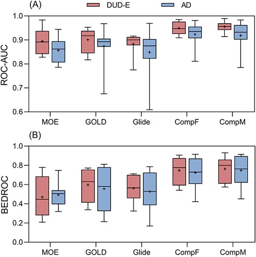
Box plot of the ROC-AUC (A) and BEDROC (B) results of five EATL SFs on eight targets of DUD-E and AD dataset. The horizontal lines indicate median, and the plus signs represent the mean value. MOE, MOE-EATL; GOLD, GOLD-EATL; and Glide, Glide-EATL. The plot is built with the values of AUC and BEDROC for all the targets as provided in Supplementary Table S4.
EATL-SFs are far superior to conventional SFs in terms of the well-established VS metrics. It was observed that EATL could highly improve the poor early recognition obtained by classical SFs across the dataset. This suggests that it’s a promising attempt to make the best use of the components provided by popular SFs to boost VS performance. We also find that complementarity exists between different scoring functions since docking-EATL SFs which use all the components within each docking program as input can obtain improved screening power. Furthermore, two comprehensive EATL models, CompF and CompM, which employ all the components from three docking programs can achieve comparably stable performance relative to other advanced ML-based SFs, suggesting that combining multiple docking programs may better compensate their individual weaknesses. Although the usefulness of rescoring aided by ML methods has already been noted, what distinguishes our method is that we make the best of conventional scoring system whose effectiveness and accuracy have been verified by extensive studies. Overall, EATL represents a new, simple and practical analytical method that not only is easy to be utilized by most VS researchers but also can be extended to other docking programs.
In addition, we notably suggest, any validation of ML-based SBVS methods on DUD-E should be cautious of the features characterizing protein–ligand interactions and make essential bias discussion on the dataset. It is impossible to require the benchmark to simulate real scenarios from all perspectives; actually, all the ML-based methods should be experimentally tested in practice. Here we encourage more adoption of our EATL strategy in the implementation of VS work and expect the development of other boosted methods and more reliable VS benchmarks that are instrumental to the community of SBVS.
Components generated from 10 scoring functions were analyzed by XGBoost algorithm to improve the screening power.
EATL-SFs, docking-EATL SFs and comprehensive SFs are superior to classical scoring functions in terms of well-established virtual screening metrics across the diverse subset of DUD-E.
Complementarity exists between different scoring functions and docking programs.
The improved VS performance of EATL could be reproduce on unbiased AD dataset.
Abbreviations
VS, virtual screening; SF, scoring functions; SBVS, structure-based virtual screening; DUD-E, Directory of Useful Decoys: Enhanced; AD, the actives as decoys; ML, machine learning; XGBoost, extreme gradient boosting; ROC-AUC, area under the receiver operating characteristic curve; EF, enrichment factor; BEDROC, Boltzmann-enhanced discrimination of receiver operating characteristic; LogAUC, log-scaled area under the receiver-operating characteristic curve.
Guo-Li Xiong is a master student at the Xiangya School of Pharmaceutical Sciences, Central South University, China. Her research focuses on the development of novel structure-based virtual screening methodologies.
Wen-Ling Ye is a master student at the Xiangya School of Pharmaceutical Sciences, Central South University, China. Her research theme is design and discovery of small molecular inhibitors of important protein targets.
Chao Shen is a PhD candidate student in the College of Pharmaceutical Sciences, Zhejiang University, China. His research interests lie in the area of computer-aided drug design.
Ai-Ping Lu is currently a professor in the Institute for Advancing Translational Medicine in Bone and Joint Diseases, School of Chinese Medicine, Hong Kong Baptist University, Hong Kong.
Ting-Jun Hou is currently a Professor in the College of Pharmaceutical Sciences, Zhejiang University, China. His research interests can be found at the website of his group: http://cadd.zju.edu.cn
Dong-Sheng Cao is currently an Associate Professor in the Xiangya School of Pharmaceutical Sciences, Central South University, China. His research interests can be found at the website of his group: http://www.scbdd.com
