A comparison and assessment of computational method for identifying recombination hotspots in Saccharomyces cerevisiae

A comprehensive list of methods for prediction recombination hotspots of S. cerevisiae

Methods	Web server	Data set	Feature extraction	Feature selection	Algorithm	Evaluation strategy
SVM-FCU	No	S1	FCU	None	SVM-RBF	10-fold CV
RF-DYMHC	Yes	S1, S2	Gapped dinucleotide composition features	None	RF	5-fold CV and Jackknife validation
IDQD-4-mer	No	S1, S2, S3	4-mer	None	IDQD	5-fold CV
IRSpot-PseDNC	Yes	S1, S2, S3	PseDNC	None	SVM-RBF	5-fold CV and Jackknife validation
SVM-NACPseDNC	No	S1	Nucleic acid composition (NAC), n-tier NAC and PseDNC	None	SVM-linear kernel	Jackknife validation
IRSpot-TNCPseAAC	Yes	S1, S2, S3	TNC and PseAAC	None	SVM-RBF	Jackknife validation
Weighted features	No	S1	k-mer, physical properties	None	Weighted features	5-fold CV
IRSpot-EL	Yes	S2	PseKNC, DACC	F-score	SVM-RBF	5-fold CV
IDQD-Nu-occ	No	S1	4-mer, Nu-occ	None	IDQD	5-fold CV
IRSpot-GAEnsC	No	S1	TNC, DNC	None	ANN + SVM + RF	Jackknife validation
HcsPredictor	Yes	S1	PseDNC+Z	None	LDM	5-fold CV and Jackknife validation
IRSpot-ADPM	No	S1, S2	ADPM	Wrapper SVM	SVM-RBF	5-fold CV and Jackknife validation
IRSpot-PDI	No	S1, S2	PDI	Wrapper SVM	SVM-RBF	Jackknife validation
IRSpot-SF	Yes	S2	Gapped dinucleotide, TF-IDF, K-mer, Reverse K-mer	SVM-RFE	SVM-RBF	5-fold CV and Jackknife validation
IRSpot-Pse6NC	Yes	S3	Pse6NC	Binomial distribution	SVM-RBF	5-fold CV

Methods	Web server	Data set	Feature extraction	Feature selection	Algorithm	Evaluation strategy
SVM-FCU	No	S1	FCU	None	SVM-RBF	10-fold CV
RF-DYMHC	Yes	S1, S2	Gapped dinucleotide composition features	None	RF	5-fold CV and Jackknife validation
IDQD-4-mer	No	S1, S2, S3	4-mer	None	IDQD	5-fold CV
IRSpot-PseDNC	Yes	S1, S2, S3	PseDNC	None	SVM-RBF	5-fold CV and Jackknife validation
SVM-NACPseDNC	No	S1	Nucleic acid composition (NAC), n-tier NAC and PseDNC	None	SVM-linear kernel	Jackknife validation
IRSpot-TNCPseAAC	Yes	S1, S2, S3	TNC and PseAAC	None	SVM-RBF	Jackknife validation
Weighted features	No	S1	k-mer, physical properties	None	Weighted features	5-fold CV
IRSpot-EL	Yes	S2	PseKNC, DACC	F-score	SVM-RBF	5-fold CV
IDQD-Nu-occ	No	S1	4-mer, Nu-occ	None	IDQD	5-fold CV
IRSpot-GAEnsC	No	S1	TNC, DNC	None	ANN + SVM + RF	Jackknife validation
HcsPredictor	Yes	S1	PseDNC+Z	None	LDM	5-fold CV and Jackknife validation
IRSpot-ADPM	No	S1, S2	ADPM	Wrapper SVM	SVM-RBF	5-fold CV and Jackknife validation
IRSpot-PDI	No	S1, S2	PDI	Wrapper SVM	SVM-RBF	Jackknife validation
IRSpot-SF	Yes	S2	Gapped dinucleotide, TF-IDF, K-mer, Reverse K-mer	SVM-RFE	SVM-RBF	5-fold CV and Jackknife validation
IRSpot-Pse6NC	Yes	S3	Pse6NC	Binomial distribution	SVM-RBF	5-fold CV

Table 1

A comprehensive list of methods for prediction recombination hotspots of S. cerevisiae

Methods	Web server	Data set	Feature extraction	Feature selection	Algorithm	Evaluation strategy
SVM-FCU	No	S1	FCU	None	SVM-RBF	10-fold CV
RF-DYMHC	Yes	S1, S2	Gapped dinucleotide composition features	None	RF	5-fold CV and Jackknife validation
IDQD-4-mer	No	S1, S2, S3	4-mer	None	IDQD	5-fold CV
IRSpot-PseDNC	Yes	S1, S2, S3	PseDNC	None	SVM-RBF	5-fold CV and Jackknife validation
SVM-NACPseDNC	No	S1	Nucleic acid composition (NAC), n-tier NAC and PseDNC	None	SVM-linear kernel	Jackknife validation
IRSpot-TNCPseAAC	Yes	S1, S2, S3	TNC and PseAAC	None	SVM-RBF	Jackknife validation
Weighted features	No	S1	k-mer, physical properties	None	Weighted features	5-fold CV
IRSpot-EL	Yes	S2	PseKNC, DACC	F-score	SVM-RBF	5-fold CV
IDQD-Nu-occ	No	S1	4-mer, Nu-occ	None	IDQD	5-fold CV
IRSpot-GAEnsC	No	S1	TNC, DNC	None	ANN + SVM + RF	Jackknife validation
HcsPredictor	Yes	S1	PseDNC+Z	None	LDM	5-fold CV and Jackknife validation
IRSpot-ADPM	No	S1, S2	ADPM	Wrapper SVM	SVM-RBF	5-fold CV and Jackknife validation
IRSpot-PDI	No	S1, S2	PDI	Wrapper SVM	SVM-RBF	Jackknife validation
IRSpot-SF	Yes	S2	Gapped dinucleotide, TF-IDF, K-mer, Reverse K-mer	SVM-RFE	SVM-RBF	5-fold CV and Jackknife validation
IRSpot-Pse6NC	Yes	S3	Pse6NC	Binomial distribution	SVM-RBF	5-fold CV

Methods	Web server	Data set	Feature extraction	Feature selection	Algorithm	Evaluation strategy
SVM-FCU	No	S1	FCU	None	SVM-RBF	10-fold CV
RF-DYMHC	Yes	S1, S2	Gapped dinucleotide composition features	None	RF	5-fold CV and Jackknife validation
IDQD-4-mer	No	S1, S2, S3	4-mer	None	IDQD	5-fold CV
IRSpot-PseDNC	Yes	S1, S2, S3	PseDNC	None	SVM-RBF	5-fold CV and Jackknife validation
SVM-NACPseDNC	No	S1	Nucleic acid composition (NAC), n-tier NAC and PseDNC	None	SVM-linear kernel	Jackknife validation
IRSpot-TNCPseAAC	Yes	S1, S2, S3	TNC and PseAAC	None	SVM-RBF	Jackknife validation
Weighted features	No	S1	k-mer, physical properties	None	Weighted features	5-fold CV
IRSpot-EL	Yes	S2	PseKNC, DACC	F-score	SVM-RBF	5-fold CV
IDQD-Nu-occ	No	S1	4-mer, Nu-occ	None	IDQD	5-fold CV
IRSpot-GAEnsC	No	S1	TNC, DNC	None	ANN + SVM + RF	Jackknife validation
HcsPredictor	Yes	S1	PseDNC+Z	None	LDM	5-fold CV and Jackknife validation
IRSpot-ADPM	No	S1, S2	ADPM	Wrapper SVM	SVM-RBF	5-fold CV and Jackknife validation
IRSpot-PDI	No	S1, S2	PDI	Wrapper SVM	SVM-RBF	Jackknife validation
IRSpot-SF	Yes	S2	Gapped dinucleotide, TF-IDF, K-mer, Reverse K-mer	SVM-RFE	SVM-RBF	5-fold CV and Jackknife validation
IRSpot-Pse6NC	Yes	S3	Pse6NC	Binomial distribution	SVM-RBF	5-fold CV

Table 2

The recombination hotspots data sets of S. cerevisiae

Benchmark data set	Data sources	Equal length	Positive subset	Negative subset
\|$\mathrm{S}$\|1[15]	Gerton et al. [1]	No	490	591
\|$\mathrm{S}$\|2[23]	Gerton et al. [1]	No	478	572
\|$\mathrm{S}3$\|[28]	Gerton et al. [1]	Yes	490	591
\|$\mathrm{S}$\|4(This paper)	Pan et al. [10]	No	3212	3202

Benchmark data set	Data sources	Equal length	Positive subset	Negative subset
\|$\mathrm{S}$\|1[15]	Gerton et al. [1]	No	490	591
\|$\mathrm{S}$\|2[23]	Gerton et al. [1]	No	478	572
\|$\mathrm{S}3$\|[28]	Gerton et al. [1]	Yes	490	591
\|$\mathrm{S}$\|4(This paper)	Pan et al. [10]	No	3212	3202

Table 2

The recombination hotspots data sets of S. cerevisiae

Benchmark data set	Data sources	Equal length	Positive subset	Negative subset
\|$\mathrm{S}$\|1[15]	Gerton et al. [1]	No	490	591
\|$\mathrm{S}$\|2[23]	Gerton et al. [1]	No	478	572
\|$\mathrm{S}3$\|[28]	Gerton et al. [1]	Yes	490	591
\|$\mathrm{S}$\|4(This paper)	Pan et al. [10]	No	3212	3202

Benchmark data set	Data sources	Equal length	Positive subset	Negative subset
\|$\mathrm{S}$\|1[15]	Gerton et al. [1]	No	490	591
\|$\mathrm{S}$\|2[23]	Gerton et al. [1]	No	478	572
\|$\mathrm{S}3$\|[28]	Gerton et al. [1]	Yes	490	591
\|$\mathrm{S}$\|4(This paper)	Pan et al. [10]	No	3212	3202

Despite the great progress made in the above research, there are still some problems. With the development of experimental technology, the resolution and sensitivity of genome-wide DSBs atlas have been greatly improved. However, the data set used in the previous models have not been improved. In previous data sets, due to the limitations of experimental methods, only DSBs within ORF can be found. However, the recombination hotspots are not limited to ORF, thus these models trained on such data set lack extensive application [11]. Furthermore, most of models did not pay attention to the problem of the sliding window size. They can only predict whether an input sequence contains recombination hotspots or not, but could not predict where the recombinant hotspots are located [27]. When a genome is scanned using a model, the question of how to set a window becomes more important.

To solve these problems, a new data set with high resolution and sensitivity was built to train a new predictor, in which the recombination hotspots are no longer limited to ORF [11]. The new model was examined on the chromosome XVI of S. cerevisiae. We believe that our work represents an important advancement in accelerating the discovery of recombination hotspots. We anticipate that our review will be helpful for future development of computational methods to efficiently and accurately identify recombination hotspots.

Methods and materials

The benchmark data sets

In 2000, Gerton et al. proposed the DNA microarray method to estimate the DSBs formation adjacent to each ORF in the S. cerevisiae at single-gene resolution. To estimate the DSBs formation adjacent to each ORF, they measured the hybridization ratio of a DSBs-enriched probe (P2) to a total genomic probe (P1) [1]. The relative strength of the recombination rate was estimated by the P2/P1 hybridization ratio. If the P2/P1 hybridization ratio ranked in the top 12.5% in more than five of seven experiments, an ORF was classified as ‘hot’, and if it ranked in the bottom 12.5%, it was classified as ‘cold’. Accordingly, the authors found 177 hotspots and 40 coldspots. In another study [13], based on Gerton et al.’s study, Jiang et al. reconstructed the data set and defined the relative hybridization ratio ≥1.5 as hotspots, while relative hybridization ratio <0.82 was defined as coldspots. Thus, Jiang et al. [13] obtained 490 hotspots and 591 coldspots, which form the training data set. The data set is called S1 and is available in Supplementary Material S1.

In Liu et al.’s study [22], to avoid redundancy and reduce homology deviations, sequences with similarity >75% were removed by using CD-HIT [28]. Then they obtained 478 hotspots and 572 coldspots, which formed data set S2 and is available in Supplementary Material S2.

It was found that the sequences in Supplementary Materials S1 and S2 are with different lengths, which prevented them from establishing a widely useful model because users do not know how long the length should be used for a query DNA sequence. Thus, an equal length data set was rebuilt [27]. The new data set, called S3, contains 490 recombination hotspots and 591 recombination coldspots with the length of 131 bp and is available in Supplementary Material S3.

In 2011, Pan et al. [11] uncovered a genome-wide DSBs map with unprecedented resolution and sensitivity by sequencing the DNA fragments that bound to accumulation of Spo11 protein covalently. Based on these data, we proposed a new data set. To avoid redundancy and reduce homology deviations [29], sequences with >75% similarity were removed using the CD-HIT procedure [28]. We obtained 3480 sequences with recombination hotspots and 3471 sequences without recombination hotspots in S. cerevisiae. Subsequently, we divided this new data set into two parts: a training data set containing sequences from chromosome I to XV and an independent test data set containing sequences from chromosome XVI. The training data set can be formulated as follows:

$$\begin{equation} \mathrm{S}={\mathrm{S}}^{+}\bigcup {\mathrm{S}}^{-},\kern9.25em \end{equation}$$

(1)

where |$\mathrm{S}$| is the benchmark data set S4, |${\mathrm{S}}^{+}$| is the positive subset containing 3212 true recombination hotspots sequences and |${\mathrm{S}}^{-}$| is the negative subset containing 3202 non-recombination hotspots sequences of S. cerevisiae in I–XV chromosomes, which are available in Supplementary Material S4. These data sets were shown in Table 2.

The independent test data set contains the remaining 268 true recombination hotspots sequences and 280 non-recombination hotspots sequences in XVI chromosomes of S. cerevisiae, which are available in Supplementary Material S5.

Feature extraction

How to formulate a biological sequence with a vector is one of the most challenging problems in computational biology [30]. This is because nearly all the existing machine learning algorithms were developed to handle vectors rather than sequence samples [31]. To capture the key information of recombination hotspots, there are two types of feature encoding algorithms that have been proposed, namely ORF-based methods and non-ORF-based methods.

ORF-based approaches

Codon use frequency

Codon use frequency (FCU) is the fusion of both codon usage bias and amino acid composition (AAC) signals [12, 32]. Each ORF was represented by a 61-dimensional vector with respect to the 61 sense codons. FCU value of the j-th codon for the i-th amino acid was calculated as follows:

$$\begin{equation} {\mathrm{FCU}}_{ij}={\mathrm{obs}}_{ij}/\mathrm{Total},\kern8.5em \end{equation}$$

(2)

where |${\mathrm{obs}}_{ij}$| is the observed number of the j-th codon for the i-th amino acid and Total is the total number of codons in the ORF.

Phase-specific PseDNC

Phase-specific PseDNC (psPseDNC) can reflect composition bias among three codon positions [21]. psPseDNC is inspired by the idea of the Z curve theory. Dong et al. [21] improved the PseDNC method to give psPseDNC. The following equations adopt a similar form to PseDNC:

$$\begin{equation} \left\{\begin{array}{@{}c}{\theta}_{1-2,\lambda }=\mathrm{mean}\left(\sum_{i\in 1}\varTheta \left({N}_i{N}_{i+1},{N}_{i+\lambda }{N}_{i+1+\lambda}\right)\right)\\ {}{\theta}_{2-3,\lambda }=\mathrm{mean}\left(\sum_{i\in 2}\varTheta \left({N}_i{N}_{i+1},{N}_{i+\lambda }{N}_{i+1+\lambda}\right)\right)\\ {}{\theta}_{3-1,\lambda }=\mathrm{mean}\left(\sum_{i\in 3}\varTheta \left({N}_i{N}_{i+1},{N}_{i+\lambda }{N}_{i+1+\lambda}\right)\right)\end{array}\right.,\kern5.25em \end{equation}$$

(3)

where |${\theta}_{1-2,\lambda }$|⁠, |${\theta}_{2-3,\lambda }$| and |${\theta}_{3-1,\lambda }$| are phase-specific order-correlated factors and reflect the sequence-order correlation. The sequence feature vectors of each DNA can be calculated using PseDNC by incorporating into |${\theta}_{1-2,\lambda }$|⁠, |${\theta}_{2-3,\lambda }$| and |${\theta}_{3-1,\lambda }$|⁠. There are three phases in a DNA sequence, therefore, a DNA sequence is now represented by|$(16+1)\times 3$| dimensional vectors.

Amino acid composition

When the sequence is ORF, we can use the AAC to extract features [18, 33, 34]. Every three bases can encode one amino acid. AAC is the frequency of each type of amino acid occurring in peptide sequences and can be calculated as follows:

$$\begin{equation} f(r)=\frac{N_r}{N},r=1,2,\dots, 20,\kern10em \end{equation}$$

(4)

where |${N}_{\mathrm{r}}$| is the number of the amino acid type |$r$| and |$N$| is the length of the sequence.

Trinucleotide composition and pseudo amino acid composition (TNCPseAAC)

TNCPseAAC is a feature extraction technique by combining trinucleotide composition [35] and pseudo amino acid composition (PseAAC) [36]. For a given gene sequence, the TNCPseAAC feature vector is represented by the following:

$$\begin{equation} \mathrm{TNCPseAAC}={\left[{d}_1{d}_2\cdots {d}_{64}{d}_{64+1}\cdots {d}_{64+\lambda -1}{d}_{64+\lambda}\right]}^{\mathrm{T}},\kern5em \end{equation}$$

(5)

where

$$\begin{equation} {d}_u=\left\{\begin{array}{@{}c}\frac{f_u}{\sum_{i=1}^{64}{f}_i+\omega {\sum}_{j=1}^{\lambda }{\theta}_j},\left(1\le u\le 64\right)\kern2em \\[8pt] {}\frac{\omega {\theta}_{u-64}}{\sum_{i=1}^{64}{f}_i+\omega {\sum}_{j=1}^{\lambda }{\theta}_j},\left(64+1\le u\le 64+\lambda \right)\end{array}\right., \end{equation}$$

(6)

where |$\omega$| is the weight factor,|${f}_u$| (1|$\le u\le 64$|⁠) represents the DNA sequence using the occurrence frequencies of its 64 trinucleotides that reflect short-range sequence-order effect, while|${\theta}_{u-64}$| reflected via the PseAAC of its translated protein chain. |${\theta}_j$|is subject to the following formula:

$$\begin{equation} {\theta}_j=\frac{1}{L^{\ast }-j}\sum_{i=1}^{L^{\ast }-j}\varTheta ({A}_i,{A}_{i+j})\quad (\lambda <{L}^{\ast }) \end{equation}$$

(7)

where |${\theta}_j(j=1,2,3,\dots, \lambda )$|is called the j-th tier correlation factor that reflects the sequence-order correlation between all the j-th most contiguous residues along a protein chain. In this study, the correlation function is given by the following:

$$\begin{equation} \varTheta \left({A}_i,{A}_j\right)= \frac{1}{6}\sum_{n-1}^6{\left[{H}_n\left({A}_j\right)-{H}_n\left({A}_i\right)\right]}^2 \end{equation}$$

(8)

where |${H}_n({A}_j)\ (n=1,2,\dots, 6)\ \mathrm{is}$| the standardized values of six physicochemical properties of amino acids. They are hydrophobicity, hydrophilicity, side-chain mass, pK1 (α-COOH), pK2 (NH3) and PI and can be obtained from Ref [18].

Non-ORF-based methods

Gapped dinucleotide composition features

The gapped dinucleotide composition uses gaps with k intervening bases between every dinucleotide within a sequence [13]. It encapsulates the composition and local order information of any two interval dinucleotides within a gene sequence rather than the adjacent dinucleotide composition. It can be defined as follows:

$$\begin{equation} {F}_{(k)}^i=\frac{o_{(k)}^i}{n_{(k)}}, \end{equation}$$

(9)

where |${o}_{(k)}^i$| is the total number of the i-th dinucleotide with k intervening bases and |${n}_{(k)}$| is the total number of all possible dinucleotide with k intervening bases. In this study, each sequence will be represented by a (⁠|${4}^2\times 2$|⁠)-dimension feature vector reflecting the dinucleotide compositions with the interval of k = 0 and k = 1.

K-mer composition

The frequency of k-mer is the ratio of the number of occurrences of the i-th k-mer in the gene sequence to the number of occurrences of all k-mer in this sequence through a window of width k sliding across the gene sequence with a step of 1 [17, 20]. We calculated the frequency of k-mer in the gene sequence according to the following equation:

$$\begin{equation} {f}_i={${n}_i$}\!\left/ \!{$\sum_{i=1}^{4^k}{n}_i$}\right.={n}_i/\left(L-k+1\right), \end{equation}$$

(10)

where |${n}_i$| denote the number of the i-th k-mer and L denotes the length of the gene sequence, respectively. When k = 2, we call this method Dinucleotide composition (DNC), and when k = 3, we call this method Trinucleotide composition (TNC). In this study, k can take the integer ranging from 1 to 8. Accordingly, each sequence can be represented as a 4^k dimensional vector.

Reverse complement composition of k-mer

The reverse complement composition of k-mer is the normalized count of k-mer and its reverse complements present in the DNA sequence [26, 37]. The difference of this feature with k-mer composition is that the reverse complement composition of k-mer counts all the occurrences of the k-mer and its reverse complement.

Term frequency–inverse document frequency of k-mer

Term frequency (TF) is the normalized frequency or composition of a string in a given sequence [26]. However, inverse document frequency (IDF) searches for k-mer that is sparsely distributed in the sequences. It is formally defined as below:

$$\begin{equation} \mathrm{IDF}\left({s}_i\right)=\log \left(\frac{\mid S\mid }{\sum_{D\in S}d\left({s}_i,D\right)}\right), \end{equation}$$

(11)

where |$\mid S\mid$| is the number of sequences in the data set S and |$d({s}_i,D)$| is a function that returns 1 if and only if the k-mer is present in the sequence D, and otherwise returns 0. TF-IDF is the multiplication of TF and IDF for each of the k-mer.

Pseudo K-tuple nucleotide composition

PseKNC method not only reflects the local sequence information of the nucleotide sequence but also describes the global sequence information of the nucleotide sequence [16, 17]. For a given gene sequence, the PseKNC feature vector is represented by:

$$\begin{equation} \mathrm{PseKNC}={\left[{d}_1{d}_2\cdots {d}_{4^k}{d}_{4^k+1}\cdots {d}_{4^k+\lambda -1}{d}_{4^k+\lambda}\right]}^{\mathrm{T}}, \end{equation}$$

(12)

where

$$\begin{equation} {d}_u=\left\{\begin{array}{@{}c}\frac{f_u}{\sum_{i=1}^{4^k}{f}_i+\omega {\sum}_{j=1}^{\lambda }{\theta}_j},\left(1\le u\le {4}^k\right)\kern2em \\[10pt] {}\frac{\omega {\theta}_{u-{4}^k}}{\sum_{i=1}^{4^k}{f}_i+\omega {\sum}_{j=1}^{\lambda }{\theta}_j},\left({4}^k+1\le u\le {4}^k+\lambda \right)\end{array}\right., \end{equation}$$

(13)

where u is an integer, |${f}_u$| (1|$\le u\le {4}^k$|⁠) represents the normalized occurrence frequency of k-mer, |$\lambda$| is the number of the total counted ranks (or tiers) of the correlations along a DNA sequence and |$\omega$| is the weight factor. |${\theta}_j$| |$(j=1,2,3,\dots, \lambda )$| is the correlation function that measures the j-tier sequence-order correlation between all the j-th most contiguous residues along sequence. |${\theta}_j$|is defined as below:

$$\begin{equation} \left\{\begin{array}{c}{\theta}_1=\frac{1}{L-k}\sum_{i=1}^{L-k}{\varTheta}_{i,i+1}\\[6pt] {}{\theta}_2=\frac{1}{L-k}\sum_{i=1}^{L-k-1}{\varTheta}_{i,i+2}\\[6pt] {}{\theta}_3=\frac{1}{L-k}\sum_{i=1}^{L-k-2}{\varTheta}_{i,i+3}\\[2pt] {}\dots \dots \\ {}{\theta}_{\lambda }=\frac{1}{L-k}\sum_{i=1}^{L-k-\lambda +1}{\varTheta}_{i,i+\lambda}\end{array}\right.\qquad (\lambda <L-k). \end{equation}$$

(14)

The parameter |$\lambda$| is an integer where|${\theta}_{\lambda }$| is called the |$\lambda$|-tier correlation factor that reflects the sequence-order correlation between all the most contiguous nucleotides along a DNA sequence and the correlation function is given by the following:

$$\begin{equation} \left\{\begin{array}{@{}c}{\varTheta}_{i,i+j}=\frac{1}{\mu}\sum_{u=1}^{\mu }{\left[{P}_u\left({R}_i{R}_{i+1}\dots {R}_{i+K-1}\right)-{P}_u\left({R}_{i+j}{R}_{i+j+1}\dots {R}_{i+j+k-1}\right)\right]}^2\\ {}j=1,2,\dots, \lambda; i=1,2,\dots, L-k-\lambda; \lambda <L-k\end{array}\right.\!\!\!, \end{equation}$$

(15)

where |$\mu$| is the number of local DNA structural properties considered. |${P}_u({R}_i{R}_{i+1}\dots {R}_{i+k-1})$|⁠, the numerical value of the u-th (u = 1,2, …,|$\mu$|⁠) DNA local property for the oligonucleotides |${R}_i{R}_{i+1}\dots {R}_{i+k-1}$| at position i and |${P}_u({R}_{i+j}{R}_{i+j+1}\dots {R}_{i+j+k-1})$|⁠, the corresponding value for the oligonucleotides |${R}_{i+j}{R}_{i+j+1}\dots {R}_{i+j+k-1}$| at position i + j. They are calculated by the following formula:

$$\begin{equation} {P}_u\left({R}_1{R}_2\dots {R}_k\right)=\frac{P_u\left({R}_1{R}_2\dots {R}_k\right)-<{P}_u\left({R}_1{R}_2\dots {R}_k\right)>}{SD<{P}_u\left({R}_1{R}_2\dots {R}_k\right)>}, \end{equation}$$

(16)

where < > represents the mean and SD represents the standard deviation. For the oligonucleotides, the original physicochemical property values can be obtained from [15]. PseDNC is a special case of k = 2 in PseKNC. k is the number of neighbouring nucleic acid residues.

Weighted features

To quantify the importance of different features in prediction and incorporate different kinds of features in a proper way, Liu et al. [20] weighted the features using a variance-based feature selection method. First, samples were represented by possibly important features, such as k-mer distribution in sequences and sequence-order-related information. Second, weights of different features were calculated according to their ability to distinguish positive samples from negative samples. Third, values of the features were normalized via a standard conversion. Finally, samples were represented by weighted features (WF) by multiplying the normalized features with their corresponding weights.

Physical properties of DNA sequences

Due to nucleosome occupancy displaying an important role in the DSBs, the influence of nucleosome occupancy on recombination spots prediction should be investigated. Fifteen physical properties of DNA sequences (Supplementary Material S6) were used to describe nucleosome and have been used in recombination spots prediction [20]. Here, we used the physical properties as features to identify recombination hotspots by the following formula:

$$\begin{equation} \left\{\begin{array}{@{}c}{h}_{n,m}=\frac{1}{L-1-n}\sum_{i=1}^{L-1-n}{\left[{P}_m\left(i,i+1\right)-{P}_m\left(i+n,i+n+1\right)\right]}^2\\ {}1<n<L-2\end{array}\right.\!\!\!\!, \end{equation}$$

(25)

where |${P}_m(i,i+1)$| and |${P}_m(i+n,i+n+1)$| denote the values of the m-th property listed in Supplementary Material S6 at dinucleotide position |$(i,i+1)$| and |$(i+n,i+n+1)$|⁠, respectively, and |$L$| is sequence length. |${h}_{n,m}$| is called the n-th tier correlation factor that reflects the sequence-order correlation with respect to the m-th parameter between all the n-th most contiguous dinucleotide along a DNA sequence.

Associated dinucleotide product model (ADPM)

ADPM is an algorithm that uses an associated dinucleotide product model to define Chou’s pseudo components [24].

For a given DNA sequence D, the ADPM feature vector is represented by:

$$\begin{equation} \mathrm{ADPM}={\left[{d}_1{d}_2\cdots {d}_u\cdots {d}_{\varOmega}\right]}^{\mathrm{T}},\kern9.25em \end{equation}$$

(17)

where

$$\begin{equation} {d}_{k,t,g}=\frac{1}{L-g-1}\sum_{i=1}^{L-g-1}{\varTheta}_{i,g,k,t},\kern8.5em \end{equation}$$

(18)

where |$k,t$| is the number of physical and chemical properties used in this study and |$k,t=1,2,\dots, 15,\kern0.5em g$| is an accumulated distance factor that determines the degree of separation between dinucleotide along the sequence. |${\varTheta}_{i,g,k,t}$| is called product operator, which is defined by the following mathematical expression:

$$\begin{equation} {\varTheta}_{i,g,k,t}={P}_{i,k}\times {P}_{i+g,t}.\kern10.75em \end{equation}$$

(19)

|${\varTheta}_{i,g,k,t}$|reflects the associated influence of dinucleotide pairs at different positions with genomic evolutionary. |${P}_{i,k}$| denotes the k-th property value of the i-th dinucleotide pair, which is composed of two adjacent nucleotides in the sequence. The given sequence can be converted into a feature vector with a uniform size of 15 × 15 ×|$g$|⁠.

Property diversity information (PDI)

PDI is an improved method of ADPM [25]. PDI reflects the property differentiation between the dinucleotide pairs in |$g$| interval along the sequence and the forward and backward order information. For a given DNA sequence D, the PDI feature vector is represented by the following:

$$\begin{equation} \mathrm{PDI}={\left[{d}_1{d}_2\cdots {d}_u\cdots {d}_{\varOmega}\right]}^{\mathrm{T}},\kern9.5em \end{equation}$$

(20)

where

$$\begin{equation} {d}_{k,t,g}=\frac{1}{L-2g-1}\sum_{i=g+1}^{L-g-1}{\varTheta}_{i,g,k,t}.\kern8.5em \end{equation}$$

(21)

The parameter in the formula is the same as (18). |${\varTheta}_{i,g,k,t}$| called diversity function is defined by the following mathematical equations:

$$\begin{equation} {\varTheta}_{i,g,k,t}={\theta}_1+{\theta}_2\kern11.5em \end{equation}$$

(22)

$$\begin{equation} {\theta}_1={\left(\frac{P_{i-g,k}-{P}_{i,t}}{2}\right)}^2\kern10.75em \end{equation}$$

(23)

$$\begin{equation} {\theta}_2={\left(\frac{P_{i,t}-{P}_{i+g,k}}{2}\right)}^2,\kern10.75em \end{equation}$$

(24)

where |${\theta}_1$| describes the differentiation between the i-th and the (i + g)-th dinucleotide according to properties t and k. Similarly, |${\theta}_2$|expresses the differentiation between the i-th and the (i-g)-th dinucleotide according to properties t and k.|${\varTheta}_{i,g,k,t}$| reflects the diversity information of dinucleotide pairs on different DNA properties with the distance g.

Dinucleotide-based auto-cross covariance

Dinucleotide-based auto-cross covariance (DACC) approach is a very special PseKNC mode, which is a combination of dinucleotide-based auto covariance and dinucleotide-based cross covariance [20].

Feature selection methods

As the dimension of the feature vector rises rapidly, we consider three issues: one is the large feature set that contains some redundant or irrelevant information; another is over-fitting, which results in low generalization ability of prediction model; the other is causing the curse of dimensionality and dyscalculia. It is necessary to employ feature selection process to improve these problems [38–40]. Three main directions have been developed for feature selection—filter, wrapper and embedded. Filters rely on the general characteristics of training data and carry out the feature selection process as a pre-processing step with independence of the induction algorithm. Wrappers involve optimizing a predictor as a part of the selection process. Embedded methods perform feature selection in the process of training and are usually specific to given learning machines. In our study, some works also use these three feature selection methods.

Binomial distribution

We should judge whether the occurrence of a particular feature is a stochastic event or not. According to the statistical theory, the binomial distribution was used to measure the occurrence probabilities of all features in positive samples and negative samples [27]. When the P value of a feature is small, the occurrence of the feature may not be a random event [41]. In this study, according to the statistical theory, the binomial distribution was used to measure the confidence of features. Then we use the incremental feature selection (IFS) to find out the best feature subset that could produce the maximum accuracy.

F-score

F-score is based on the idea that the differences within classes should be less than the differences between classes [42]. The larger the F-score value, the greater the difference between this feature and other features. It also indicates that the feature has stronger discrimination and greater effect on the prediction result. Specific implementation methods can be seen in a recent study [20].

Wrapper SVM

In this study, a wrapper feature selection process with SVM classifier is performed. Specifically, sequential forward selection strategy is adopted, in which features are sequentially added one by one to an empty candidate set until the addition of further features does not increase the criterion [25]. The criterion is defined by the overall accuracy obtained from SVM with n-fold cross-validation (CV). Finally, an optimal feature subset was constructed.

Recursive feature elimination for support vector machines

Recursive Feature Elimination for Support Vector Machines (SVM-RFE) was applied to select a group of important features [43]. This embedded method performs feature selection by iteratively training an SVM classifier with the current set of features and removing the least important feature indicated by the SVM [17, 26].

Model training

Support vector machine

SVM is a type of supervised machine learning algorithm. It has been successfully applied in the field of bioinformatics [44–50]. The basic idea of SVM is to transform the data into a high-dimensional feature space and then determine the optimal separating hyperplane. The choice of SVM kernel function plays a crucial role in the performance. Commonly used kernel functions are linear kernel function, polynomial kernel function, Radial Basis Function (RBF) kernel functions and sigmoid kernel function. Some software packages have been developed for the implication of SVM, such as LIBSVM, mySVM and SVMLight [51, 52]. In the SVM operation engine, the grid search method was applied to optimize the regularization parameter C and kernel parameter γ in the following ranges:

$$\begin{equation} \left\{\begin{array}{c}{2}^{-5}\le C\le {2}^{15}\kern1.5em \mathrm{with}\ \mathrm{step}\ \Delta C=2\\ {}{2}^{-15}\le \gamma \le {2}^{-5}\kern1.5em \mathrm{with}\ \mathrm{step}\ \Delta \gamma ={2}^{-1}\end{array}\right.\!\!.\kern5.5em \end{equation}$$

(25)

Random forest

The RF algorithm is also a popular machine learning algorithm and has been successfully employed in dealing with various biological prediction problems [53–55]. RF is a classifier that contains multiple decision trees; it is adopted bagging and random feature selection strategy. In bagging, each tree is trained on a bootstrap sample of the training data, and predictions are made by the majority votes of trees. RF is a further development of bagging. Instead of using all features, RF randomly selects a subset of features to split at each node when growing a tree. To assess the prediction performance of the algorithm, RF performs a type of cross-validation in parallel with the training step by using the so-called out-of-bag samples [56]. The RF algorithm was implemented by the Random Forest R package [13].

Recently, Ke et al. [57] proposed a novel RF algorithm named LightGBM, which uses a novel gradient boosting decision tree algorithm, including gradient-based one-side sampling to extract relatively small number of samples according to gradient values and exclusive feature bundling to reduce the number of features.

Increment of diversity

In bioinformatics, the increment of diversity (ID) method is widely applied to the prediction of sequences, structures and functions [58, 59]. Given the two diversity sources |$X=\{{x}_1,{x}_2,\dots, {x}_n\}$| and |$Y=\{{y}_1,{y}_2,\dots, {y}_n\}$|⁠, ID is defined as follows:

$$\begin{equation} ID\left(X,Y\right)=D\left(X+Y\right)-D(X)-D(Y)\kern8.75em \end{equation}$$

(26)

$$\begin{equation} D(X)= NlnN-\sum_{i=1}^d{n}_i\mathit{\ln}{n}_i\kern10.25em \end{equation}$$

(27)

$$\begin{equation} D(Y)= MlnM-\sum_{i=1}^d{m}_i\mathit{\ln}{m}_i,\kern9.75em \end{equation}$$

(28)

where |$N={\sum}_{i=1}^d{n}_i,M={\sum}_{i=1}^d{m}_i,{n}_i$| and |${m}_i$| indicate the absolute frequency of the i-th state in diversity source X and Y, respectively. |$D(X+Y)$| is the diversity measure of the mixed source |$X+Y$|⁠:|$\{{x}_1+{y}_1,{x}_2+{y}_2,\dots, {x}_n+{y}_n\}$|⁠. Diversity measure is a description of total uncertainty of information in a state space, and the ID quantitatively describes the similarity level of two diversity sources. The smaller the ID, the higher the similarity between the two corresponding diversity sources.

Quadratic discriminant

In Liu’s study [60], a quadratic discriminant (QD) function based on Mahalanobis distance was used for prediction of recombination hotspots [60]. Mahalanobis distance is based on correlations between variables by which different patterns can be identified and analysed. It is a useful measure of difference between an unknown sample set and a known one. The combination of ID and QD algorithms led to a powerful classifier called IDQD.

Large margin distribution machine

The margin distribution has a crucial influence on the performance of classifiers. Large margin distribution machine (LDM), which is inspired by the generalization performance can be improved by optimizing the margin distribution through maximizing the margin mean and minimizing the margin variance simultaneously [21, 61]. Using LDM to implement classification generally requires two steps: first, mapping the feature vector to the high-dimensional space; second, using the hyperplane to maximize the margin mean while minimizing the margin variance, thereby conveniently separating the samples. There are two solvers in the LDM: the dual coordinate descent method and the average stochastic gradient descent method. In our study, we use the dual coordinate descent method.

Artificial neural network

Artificial neural network (ANN) abstracts the human brain neuron network from the perspective of information processing, establishes a simple model and forms different networks according to different connection methods. In the past decade or so, the research work of ANNs has been deepened and great progress has been made. It has been successfully applied in the field of bioinformatics [62, 63]. In this research [23], a variety of ANN methods have also been applied, such as probabilistic neural network, generalize regression neural network, feed forward neural network, fitting network and pattern recognition network.

K-nearest neighbour (KNN)

KNN is a widely used algorithm in the field of pattern recognition [23]. The flexibility of KNN is of great advantage for gene function classification problems, wherein the class boundaries are inherently vague, and many classes cannot be categorized by a simple model. The main idea of the classical KNN is the following: design a set of numerical features to describe each data point and select a metric, e.g. Euclidean distance, to measure the similarity of data points based on all features. Then for a target point, find its K closest points in the training samples based on the similarity metric and assign it to a class by the majority votes of its neighbours.

Table 3

Comparison with state-of-the-art predictors on data sets S1

Methods	5-fold cross-validation				Jackknife validation
Methods	Sn(%)	Sp(%)	Acc(%)	MCC	Sn(%)	Sp(%)	Acc(%)	MCC
RF-DYMHC	80.59	84.26	82.05	0.638	–	–	–	–
IDQD-4-mer	79.40	81.00	80.30	0.603	–	–	–	–
IRSpot-PseDNC	81.63	88.14	85.19	0.692	73.06	89.49	82.04	0.638
SVM-NACPseDNC	–	–	–	–	76.12	90.69	84.09	0.680
IRSpot-TNCPseAAC	–	–	–	–	84.17	79.59	83.72	0.671
Weighted-Features	86.10	94.30	90.70	0.812	–	–	–	–
IDQD-Nu-occ	80.00	82.90	81.60	0.629	–	–	–	–
IRSpot-GAEnsC	–	–	–	–	80.08	88.07	84.46	0.690
HcsPredictor	77.82	89.78	84.36	0.685	78.78	90.69	85.29	0.704
ANN-AAC	–	–	–	–	–	–	–	–
IRSpot-ADPM	–	–	–	–	75.51	90.52	83.72	0.673
IRSpot-PDI	–	–	–	–	71.63	93.91	83.81	0.681

Methods	5-fold cross-validation				Jackknife validation
Methods	Sn(%)	Sp(%)	Acc(%)	MCC	Sn(%)	Sp(%)	Acc(%)	MCC
RF-DYMHC	80.59	84.26	82.05	0.638	–	–	–	–
IDQD-4-mer	79.40	81.00	80.30	0.603	–	–	–	–
IRSpot-PseDNC	81.63	88.14	85.19	0.692	73.06	89.49	82.04	0.638
SVM-NACPseDNC	–	–	–	–	76.12	90.69	84.09	0.680
IRSpot-TNCPseAAC	–	–	–	–	84.17	79.59	83.72	0.671
Weighted-Features	86.10	94.30	90.70	0.812	–	–	–	–
IDQD-Nu-occ	80.00	82.90	81.60	0.629	–	–	–	–
IRSpot-GAEnsC	–	–	–	–	80.08	88.07	84.46	0.690
HcsPredictor	77.82	89.78	84.36	0.685	78.78	90.69	85.29	0.704
ANN-AAC	–	–	–	–	–	–	–	–
IRSpot-ADPM	–	–	–	–	75.51	90.52	83.72	0.673
IRSpot-PDI	–	–	–	–	71.63	93.91	83.81	0.681

Table 3

Comparison with state-of-the-art predictors on data sets S1

Methods	5-fold cross-validation				Jackknife validation
Methods	Sn(%)	Sp(%)	Acc(%)	MCC	Sn(%)	Sp(%)	Acc(%)	MCC
RF-DYMHC	80.59	84.26	82.05	0.638	–	–	–	–
IDQD-4-mer	79.40	81.00	80.30	0.603	–	–	–	–
IRSpot-PseDNC	81.63	88.14	85.19	0.692	73.06	89.49	82.04	0.638
SVM-NACPseDNC	–	–	–	–	76.12	90.69	84.09	0.680
IRSpot-TNCPseAAC	–	–	–	–	84.17	79.59	83.72	0.671
Weighted-Features	86.10	94.30	90.70	0.812	–	–	–	–
IDQD-Nu-occ	80.00	82.90	81.60	0.629	–	–	–	–
IRSpot-GAEnsC	–	–	–	–	80.08	88.07	84.46	0.690
HcsPredictor	77.82	89.78	84.36	0.685	78.78	90.69	85.29	0.704
ANN-AAC	–	–	–	–	–	–	–	–
IRSpot-ADPM	–	–	–	–	75.51	90.52	83.72	0.673
IRSpot-PDI	–	–	–	–	71.63	93.91	83.81	0.681

Methods	5-fold cross-validation				Jackknife validation
Methods	Sn(%)	Sp(%)	Acc(%)	MCC	Sn(%)	Sp(%)	Acc(%)	MCC
RF-DYMHC	80.59	84.26	82.05	0.638	–	–	–	–
IDQD-4-mer	79.40	81.00	80.30	0.603	–	–	–	–
IRSpot-PseDNC	81.63	88.14	85.19	0.692	73.06	89.49	82.04	0.638
SVM-NACPseDNC	–	–	–	–	76.12	90.69	84.09	0.680
IRSpot-TNCPseAAC	–	–	–	–	84.17	79.59	83.72	0.671
Weighted-Features	86.10	94.30	90.70	0.812	–	–	–	–
IDQD-Nu-occ	80.00	82.90	81.60	0.629	–	–	–	–
IRSpot-GAEnsC	–	–	–	–	80.08	88.07	84.46	0.690
HcsPredictor	77.82	89.78	84.36	0.685	78.78	90.69	85.29	0.704
ANN-AAC	–	–	–	–	–	–	–	–
IRSpot-ADPM	–	–	–	–	75.51	90.52	83.72	0.673
IRSpot-PDI	–	–	–	–	71.63	93.91	83.81	0.681

Performance evaluation

In order to measure the prediction quality, the following set of four metrics was used: sensitivity (Sn), specificity (Sp), overall accuracy (Acc) and Matthews correlation coefficient (MCC) [64–69].

Sn and Sp indicate the ability to correctly identify recombination hotspot and non-recombination hotspot, respectively. Acc is the overall accuracy describing the discrimination between recombination hotspot and non-recombination hotspot. MCC can be intuitive to measure a binary classification problem. These measures are defined as follows:

$$\begin{equation} \left\{\begin{array}{c} Sn=1-\frac{N_{-}^{+}}{N^{+}}\kern6.75em 0\le Sn\le 1\\[5pt] {} Sp=1-\frac{N_{+}^{-}}{N^{-}}\kern6.75em 0\le Sp\le 1\\[5pt] {} Acc=1-\frac{N_{-}^{+}+{N}_{+}^{-}}{N^{+}+{N}^{-}}\kern5.25em 0\le Acc\le 1\\[5pt] {}\kern0.75em MCC=\frac{1-\left(\frac{N_{-}^{+}}{N^{+}}+\frac{N_{+}^{-}}{N^{-}}\right)}{\sqrt{\left(1+\frac{N_{+}^{-}-{N}_{-}^{+}}{N^{+}}\right)\left(1+\frac{N_{-}^{+}-{N}_{+}^{-}}{N^{-}}\right)}}\kern1.25em 0\le MCC\le 1,\end{array}\right.\kern2em \end{equation}$$

(29)

where |${N}^{+}$| is the total number of the positive samples investigated, while |${N}_{-}^{+}$| is the number of positive samples incorrectly predicted as the negative samples; |${N}^{-}$|is the total number of the negative samples sequence investigated, while |${N}_{+}^{-}$|is the number of the negative samples incorrectly predicted as the positive samples.

Receiver operating characteristic curve

The receiver operating characteristic (ROC) curve [70–74] was also used to measure the prediction power of the current method, where its vertical coordinate is for the true positive rate (⁠|$\mathrm{Sensitivity}$|⁠) and the horizontal coordinate for the false positive rate (⁠|$1-\mathrm{Specificity}$|⁠). The area under the curve of ROC (AUC) of 0.5 is equivalent to random prediction, while a value of 1 represents a perfect one.

Table 4

Comparison with state-of-the-art predictors on data sets S2

Methods	5-fold cross-validation				Jackknife cross-validation
Methods	Sn(%)	Sp(%)	Acc(%)	MCC	Sn(%)	Sp(%)	Acc(%)	MCC
iRSpot-EL	75.29	88.81	82.65	0.651	–	–	–	–
RF-DYMHC	73.01	86.56	80.40	0.605	–	–	–	–
IDQD-4-mer	79.52	81.82	80.77	0.616	–	–	–	–
IRSpot-PseDNC	71.75	85.84	79.33	0.583	–	–	–	–
IRSpot-TNCPseAAC	76.56	70.99	73.52	0.474	–	–	–	–
IRSpot-ADPM	77.19	90.73	84.57	0.690	76.36	90.56	84.10	0.681
IRSpot-PDI	71.84	92.95	83.16	0.666	–	–	–	–
iRSpot-SF	84.57	75.76	84.58	0.694	75.31	91.08	83.91	0.677

Methods	5-fold cross-validation				Jackknife cross-validation
Methods	Sn(%)	Sp(%)	Acc(%)	MCC	Sn(%)	Sp(%)	Acc(%)	MCC
iRSpot-EL	75.29	88.81	82.65	0.651	–	–	–	–
RF-DYMHC	73.01	86.56	80.40	0.605	–	–	–	–
IDQD-4-mer	79.52	81.82	80.77	0.616	–	–	–	–
IRSpot-PseDNC	71.75	85.84	79.33	0.583	–	–	–	–
IRSpot-TNCPseAAC	76.56	70.99	73.52	0.474	–	–	–	–
IRSpot-ADPM	77.19	90.73	84.57	0.690	76.36	90.56	84.10	0.681
IRSpot-PDI	71.84	92.95	83.16	0.666	–	–	–	–
iRSpot-SF	84.57	75.76	84.58	0.694	75.31	91.08	83.91	0.677

Table 4

Comparison with state-of-the-art predictors on data sets S2

Methods	5-fold cross-validation				Jackknife cross-validation
Methods	Sn(%)	Sp(%)	Acc(%)	MCC	Sn(%)	Sp(%)	Acc(%)	MCC
iRSpot-EL	75.29	88.81	82.65	0.651	–	–	–	–
RF-DYMHC	73.01	86.56	80.40	0.605	–	–	–	–
IDQD-4-mer	79.52	81.82	80.77	0.616	–	–	–	–
IRSpot-PseDNC	71.75	85.84	79.33	0.583	–	–	–	–
IRSpot-TNCPseAAC	76.56	70.99	73.52	0.474	–	–	–	–
IRSpot-ADPM	77.19	90.73	84.57	0.690	76.36	90.56	84.10	0.681
IRSpot-PDI	71.84	92.95	83.16	0.666	–	–	–	–
iRSpot-SF	84.57	75.76	84.58	0.694	75.31	91.08	83.91	0.677

Methods	5-fold cross-validation				Jackknife cross-validation
Methods	Sn(%)	Sp(%)	Acc(%)	MCC	Sn(%)	Sp(%)	Acc(%)	MCC
iRSpot-EL	75.29	88.81	82.65	0.651	–	–	–	–
RF-DYMHC	73.01	86.56	80.40	0.605	–	–	–	–
IDQD-4-mer	79.52	81.82	80.77	0.616	–	–	–	–
IRSpot-PseDNC	71.75	85.84	79.33	0.583	–	–	–	–
IRSpot-TNCPseAAC	76.56	70.99	73.52	0.474	–	–	–	–
IRSpot-ADPM	77.19	90.73	84.57	0.690	76.36	90.56	84.10	0.681
IRSpot-PDI	71.84	92.95	83.16	0.666	–	–	–	–
iRSpot-SF	84.57	75.76	84.58	0.694	75.31	91.08	83.91	0.677

Model validation method

Cross-validation is a commonly used statistical analysis method that can be used to objectively evaluate the performance of a classification model [75, 76]. There are three commonly used cross-validation methods, namely independent data set test, n-fold cross-validation test and jackknife cross-validation test. To objectively evaluate the performance of different models, we tested them on the independent test data sets in this review.

Results and discussion

Comparison with state-of-the-art predictors on four data sets

Considering the fact that the existing methods were trained and tested based on different data, we evaluated them on data sets S1, S2, S3 and S4, respectively.

We firstly evaluated the 12 predictors that trained based on data set S1 and listed results in Table 3. Their results are based on the 5-fold cross-validation test and jackknife test. It can be seen that the model WF performs the best in 5-fold cross-validation test and got the best Sn/Sp/Acc/Mcc. WF is developed by using QD analysis based on WF. This result demonstrates that weighting the importance of the feature is effective for improving the accuracy of the model. In the jackknife test, the best result is obtained by the model of HcsPredictor. We also noticed that the model iRSpot-GAEnsC that integrates seven algorithms did not improve the prediction accuracy of the model. Therefore, we should cautiously choose the integration approach.

Eight predictors are based on the data set S2. As shown in Table 4, iRSpot-ADPM is the best predictor in 5-fold cross-validation. IRSpot-ADPM used the weights calculated by the SVM method to decrease features from 1575 to 85. After that, support vector machine-Gaussian radial basis function (SVM-RBF) is verified by 5-fold cross-validation and obtained an accuracy of 84.57%. Compared with the accuracy of 83.14% obtained by the iRSpot-ADPM1575, iRSpot-ADPM employed fewer features but obtained higher accuracy. So it can be understood that feature filtering is very helpful for building a model with a subset of non-redundant features.

Data set S3 is an isometric data set based on data set S1. Data set S3 can easily form a window to scan the entire sequence. This kind of predictor is more applicable, which is very important for discovering new recombination hotspots. As shown in Table 5, based on data set S3, the predictor iRSpot-Pse6NC achieved the best results.

Table 5

Comparison with state-of-the-art predictors on data sets S3 in 5-fold cross-validation

Methods	Sn(%)	Sp(%)	Acc(%)	MCC
IRSpot-Pse6NC	75.71	91.03	84.08	0.6805
IRSpot-PseDNC	62.34	90.52	77.92	0.5585
IRSpot-TNCPseAAC	61.02	89.51	76.60	0.5334
IDQD-4-mer	69.59	75.09	72.59	0.4469

Methods	Sn(%)	Sp(%)	Acc(%)	MCC
IRSpot-Pse6NC	75.71	91.03	84.08	0.6805
IRSpot-PseDNC	62.34	90.52	77.92	0.5585
IRSpot-TNCPseAAC	61.02	89.51	76.60	0.5334
IDQD-4-mer	69.59	75.09	72.59	0.4469

Table 5

Comparison with state-of-the-art predictors on data sets S3 in 5-fold cross-validation

Methods	Sn(%)	Sp(%)	Acc(%)	MCC
IRSpot-Pse6NC	75.71	91.03	84.08	0.6805
IRSpot-PseDNC	62.34	90.52	77.92	0.5585
IRSpot-TNCPseAAC	61.02	89.51	76.60	0.5334
IDQD-4-mer	69.59	75.09	72.59	0.4469

Methods	Sn(%)	Sp(%)	Acc(%)	MCC
IRSpot-Pse6NC	75.71	91.03	84.08	0.6805
IRSpot-PseDNC	62.34	90.52	77.92	0.5585
IRSpot-TNCPseAAC	61.02	89.51	76.60	0.5334
IDQD-4-mer	69.59	75.09	72.59	0.4469

Based on data set S4 containing both ORF and non-ORF recombination hotspots, we construct a predictor called iRSpot-Pse6NC2.0 by incorporating the key hexamer features into the general PseKNC via the binomial distribution feature selection approach. We sorted the features according to the scores obtained from binomial distribution. By using overall accuracy as vertical coordinates and feature numbers as horizontal coordinates, we plotted IFS curve as shown in Figure 1. It was noticed that the peak of the curve is 77.61%, which is located at horizontal coordinate of 1000. This result (77.61%) is higher than that (74.85%) by using all features. Accordingly, the 1000 hexamers were selected to form the optimal feature subset to train the prediction model.

Figure 1

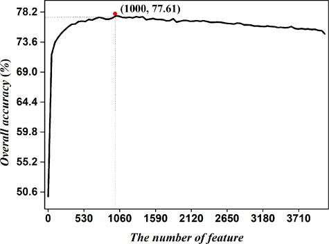
IFS curve for predicting recombination hotspots based on the 5-fold cross-validation. An IFS peak of 77.61% was observed when using the top 1000 hexamers to perform prediction

To further investigate the performance of the iRSpot-Pse6NC2.0, we drew the ROC curve in Figure 2. It shows that the AUC reaches a value of 0.833, indicating that the proposed method is quite promising and holds very high potential to become a useful high-throughput tool for predicting recombination hotspots.

Figure 2

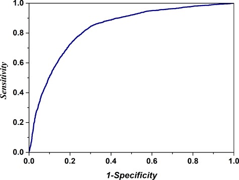
The ROC curve for identifying recombination hotspots by using 1000 optimal hexamers. The AUC of 0.833 was obtained in 5-fold cross-validation. The diagonal dot line denotes a random guess with the AUC of 0.5

Comparison with physical properties

In S. cerevisiae, both proteins Set1 and Spo11 affect the formation of DSBs through specific binding of DNA sequences [77, 78]. As a sequence feature, the hexamer can reflect the influence of these two proteins on the formation of DSBs. Due to nucleosome occupancy displaying an important role in the DSBs, we further investigated the influence of nucleosome occupancy on recombination spots prediction by adding feature of physical properties of nucleosome [20]. As it can be seen from Table 6, the nucleosome feature could produce the accuracy of 74.74%, demonstrating that the nucleosomes could influence the recombination. However, by combining the nucleosome feature with optimal hexamer composition, the accuracy reduced to 74.20%, suggesting that there is information redundancy. In fact, many studies have shown that hexamer composition is an important feature that could describe DNA motifs and could be utilized to identify a variety of DNA regulatory elements [77, 79]. Our results exactly reflected this property. The maximum accuracy of 77.61% was obtained by the optimal hexamers.

Table 6

Comparison with physical properties on data set S4

Feature	Algorithm	5-fold cross-validation
Feature	Algorithm	Sn(%)	Sp(%)	Acc(%)
Optimal hexamers	SVM	75.24	78.01	77.611
Optimal hexamers	LightGBM	77.24	75.80	76.531
Physical properties	SVM	72.91	74.89	74.742
Optimal hexamers & Physical properties	SVM	73.59	74.79	74.197

Feature	Algorithm	5-fold cross-validation
Feature	Algorithm	Sn(%)	Sp(%)	Acc(%)
Optimal hexamers	SVM	75.24	78.01	77.611
Optimal hexamers	LightGBM	77.24	75.80	76.531
Physical properties	SVM	72.91	74.89	74.742
Optimal hexamers & Physical properties	SVM	73.59	74.79	74.197

Table 6

Comparison with physical properties on data set S4

Feature	Algorithm	5-fold cross-validation
Feature	Algorithm	Sn(%)	Sp(%)	Acc(%)
Optimal hexamers	SVM	75.24	78.01	77.611
Optimal hexamers	LightGBM	77.24	75.80	76.531
Physical properties	SVM	72.91	74.89	74.742
Optimal hexamers & Physical properties	SVM	73.59	74.79	74.197

Feature	Algorithm	5-fold cross-validation
Feature	Algorithm	Sn(%)	Sp(%)	Acc(%)
Optimal hexamers	SVM	75.24	78.01	77.611
Optimal hexamers	LightGBM	77.24	75.80	76.531
Physical properties	SVM	72.91	74.89	74.742
Optimal hexamers & Physical properties	SVM	73.59	74.79	74.197

We also analysed the top 50 hexamer features that had the greatest impact on the results and found that the proportion of AT-content in these hexamers were relatively high. In S. cerevisiae, although recombination hotspots and GC-content at longer ranges were positively correlated, studies have found that many recombination spots are mostly in intergenic regions, which tend to be more at AT-rich than their surrounding regions [11].

Availability of online web server

For the convenience of the vast majority of experimental scientists, an online service is usually built. Users only need to submit the data in FASTA format to complete the prediction. Among the 15 existing predictors, only seven of them provide the online service. After checking them, as shown in Table 7, we found that only four web servers can be used at present.

Table 7

The URL addresses for the listed tools

Methods	Webservers	Available or not
iRSpotPseDNC	http://lin-group.cn/server/iRSpot-PseDNC	Yes
iRSpot-pse6NC	http://lin-group.cn/server/iRSpot-pse6NC/	Yes
iRSpot-SF	http://irspot.pythonanywhere.com/server	No
RF-DYMHC	http://www.bioinf.seu.edu.cn/Recombination/	No
HcsPredictor	http://cefg.cn/HcsPredictor	No
iRSpot-EL	http://bioinformatics.hitsz.edu.cn/iRSpot-EL/	Yes
iRSpot-TNCPseAAC	http://www.jci-bioinfo.cn/iRSpot-TNCPseAAC	Yes

Methods	Webservers	Available or not
iRSpotPseDNC	http://lin-group.cn/server/iRSpot-PseDNC	Yes
iRSpot-pse6NC	http://lin-group.cn/server/iRSpot-pse6NC/	Yes
iRSpot-SF	http://irspot.pythonanywhere.com/server	No
RF-DYMHC	http://www.bioinf.seu.edu.cn/Recombination/	No
HcsPredictor	http://cefg.cn/HcsPredictor	No
iRSpot-EL	http://bioinformatics.hitsz.edu.cn/iRSpot-EL/	Yes
iRSpot-TNCPseAAC	http://www.jci-bioinfo.cn/iRSpot-TNCPseAAC	Yes

Table 7

The URL addresses for the listed tools

Methods	Webservers	Available or not
iRSpotPseDNC	http://lin-group.cn/server/iRSpot-PseDNC	Yes
iRSpot-pse6NC	http://lin-group.cn/server/iRSpot-pse6NC/	Yes
iRSpot-SF	http://irspot.pythonanywhere.com/server	No
RF-DYMHC	http://www.bioinf.seu.edu.cn/Recombination/	No
HcsPredictor	http://cefg.cn/HcsPredictor	No
iRSpot-EL	http://bioinformatics.hitsz.edu.cn/iRSpot-EL/	Yes
iRSpot-TNCPseAAC	http://www.jci-bioinfo.cn/iRSpot-TNCPseAAC	Yes

Methods	Webservers	Available or not
iRSpotPseDNC	http://lin-group.cn/server/iRSpot-PseDNC	Yes
iRSpot-pse6NC	http://lin-group.cn/server/iRSpot-pse6NC/	Yes
iRSpot-SF	http://irspot.pythonanywhere.com/server	No
RF-DYMHC	http://www.bioinf.seu.edu.cn/Recombination/	No
HcsPredictor	http://cefg.cn/HcsPredictor	No
iRSpot-EL	http://bioinformatics.hitsz.edu.cn/iRSpot-EL/	Yes
iRSpot-TNCPseAAC	http://www.jci-bioinfo.cn/iRSpot-TNCPseAAC	Yes

Performance comparison on the yeast chromosome XVI

If the input sequence is too long, there will be two problems. One is that it cannot achieve a good prediction effect; the other is that it cannot predict whether the sequence contains multiple recombinant hotspots. In order to solve this problem, some predictors introduce sliding window method, which is to use sliding window scanning the input sequences and then predict the sub-sequence. There are two kinds of methods for the implementation of sliding window. One is iRSpot-Pse6NC, where in the model is built from the equal-length data set. When the prediction is made, the input sequence is divided into sub-sequences with the same length as that in the training data set. Another is iRSpot-EL. In the predictor, the input sequence is segmented according to the length of the window set by the user, and then the generated sub-sequence is predicted. Both methods have their own advantages. iRSpot-Pse6NC determines the most appropriate window length, while iRSpot-EL retains the complete experimental data as the training set. In newly constructed predictor iRSpot-Pse6NC2.0, we combined the above two advantages, retained complete experimental data to construct the training set and took the average length of sequence as the length of sliding window (189 bp).

Then, we used the yeast chromosome XVI to compare the performance of the predictors. We submitted the yeast chromosome XVI in FASTA format to the web servers listed in Table 7 and iRSpot-Pse6NC2.0 to obtain corresponding prediction results.

The predictor iRSpot-PseDNC and iRSpot-TNCPseAAC could not predict chromosome XVI directly, because the whole chromosome sequence is too long to be predicted. The predictor iRSpot-EL cannot be implemented according to the preset parameters. The predictor iRSpot-pse6NC segmented the chromosome according to the window length of 131 bp to generate sub-sequence and then obtained the results of sub-sequence. iRSpot-Pse6NC2.0 segmented the chromosome in a window length of 189 bp with the step of 189 bp. Then, we analysed the prediction results of iRSpot-Pse6NC and iRSpot-Pse6NC2.0. As shown in Figure 3, the average result of iRSpot-Pse6NC2.0 (Figure 3A) is higher than iRSpot-Pse6NC(Figure 3B), indicating that it is important to accurately predict the recombination hotspot region to retain the complete experimental data as the training set.

Figure 3

The prediction accuracy of (A) iRSpot-Pse6NC2.0 and (B) iRSpot-Pse6NC on the chromosome XVI.

In order to provide a detail analysis, we sorted the prediction probability of the 268 recombination hotspots that have been experimentally confirmed in a descending order. Then we used each prediction probability values as a threshold and calculated the number of sub-sequences with an accuracy greater than the threshold; the detailed results are shown in Figure 4. From Figures 3A and 4A, 220 experimentally verified recombination hotspots were correctly identified with an accuracy of 82.10% (220/268) and 1111 additional predictions were obtained by iRSpot-Pse6NC2.0. As indicated in Figures 3B and 4B, 109 experimentally verified recombination hotspots were correctly identified with an accuracy of 40.67% (109/268) and 1084 additional predictions were obtained by iRSpot-Pse6NC. These results demonstrate that the iRSpot-Pse6NC2.0 is more credible, reliable and robust for finding potential recombination hotspots.

Figure 4

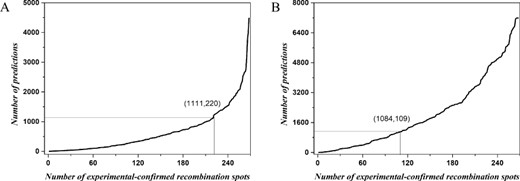
Prediction results of (A) iRSpot-Pse6NC2.0 and (B) iRSpot-Pse6NC on the chromosome XVI.

Performance analysis on the independent data set

We further compared the prediction performance of our proposed iRSpot-Pse6NC2.0 with that of iRSpot-PseDNC and iRSpot-TNCPseAAC based on the independent data set. The comparative results were listed in Table 8. The accuracy of iRSpot-PseDNC and iRSpot-TNCPseAAC was 56.16% and 54.58%，respectively, which is lower than 77.43% obtained by iRSpot-Pse6NC2.0, indicating that iRSpot-Pse6NC2.0 is better than iRSpot-TNCPseAAC and iRSpotPseDNC. This may be due to the fact that iRSpot-TNCPseAAC and iRSpotPseDNC were trained based on ORF data, while the data set of iRSpot-Pse6NC2.0 were constructed based on the data derived from the entire chromosome. The hexamer feature used in iRSpot-Pse6NC2.0 was obtained from DNA sequences directly. Thus, the model is more flexible.

Table 8

Comparison with state-of-the-art predictors on independent data set S4

Methods	Sn(%)	Sp(%)	Acc(%)
iRSpot-PseDNC	76.86	35.44	56.16
iRSpot-TNCPseAAC	56.34	52.61	54.48
iRSpot-Pse6NC2.0	77.23	77.61	77.43

Table 8

Comparison with state-of-the-art predictors on independent data set S4

Methods	Sn(%)	Sp(%)	Acc(%)
iRSpot-PseDNC	76.86	35.44	56.16
iRSpot-TNCPseAAC	56.34	52.61	54.48
iRSpot-Pse6NC2.0	77.23	77.61	77.43

Conclusion

Meiotic recombination has important roles in genome diversity and evolution, which is one of the most important driving forces of evolution. Investigations on recombination events and especially identification of recombination hotspots are significant for understanding the mechanism of recombination initiation. Since the drawbacks of experimental methods, computational methods will assist to identify recombination hotspots in a more efficient way. In this work, we have introduced and comprehensively evaluated the currently available tools for the prediction of recombination hotspots in S. cerevisiae. These computational methods were discussed and compared in terms of underlying algorithms, extracted features, predictive capability and practical utility. Subsequently, a new predictor called iRSpot-Pse6NC2.0 was constructed based on a more objective benchmark data set. To obtain a more objective performance evaluation, we constructed an independent test data set to benchmark all tools. The results demonstrated that the new predictor iRSpot-Pse6NC2.0 is superior to existing tools in the identification of recombination hotspots. We anticipate that iRSpot-Pse6NC2.0 available at http://lin-group.cn/server/iRSpot-Pse6NC2.0 will become a powerful tool for identifying recombination hotspots.

It should be noted that the proposed model iRSpot-Pse6NC2.0 was constructed based on a single-cell organism (S. cerevisiae) data. Due to species specificity, it may not be suitable for higher eukaryotes. However, the model can be used in other fungal genomes. In fact, species specificity is an important factor affecting the prediction performance of proposed models, so more and more bioinformatics models have been constructed for species specificity prediction [80, 81]. In the future, with the accumulation of higher eukaryotes data, we will update our model, which will be suitable for more species.

Key Points

A total of 15 computational methods developed for identifying recombination hotspots were comprehensively summarized and discussed.
Several comparisons were performed to investigate the predictive capability of published methods.
A high-quality data set was built to train and test a new prediction model for identifying recombination hotspots.
A user-friendly web server was developed to recognize recombination hotspots.

Funding

This work was supported by the National Nature Scientific Foundation of China (61772119, 31771471, 61861036) and the Science Strength Promotion Programme of UESTC.

Hui Yang is a PhD candidate at the Center for Informational Biology, University of Electronic Science and Technology of China. Her research interests are bioinformatics, machine learning, RNA modification site and recombination spots.

Wuritu Yang is an associate professor at the State Key Laboratory of Reproductive Regulation and Breeding of Grassland Livestock, Inner Mongolia University. His research is in the areas of bioinformatics.

Fu-Ying Dao is a PhD candidate at the Center for Informational Biology, University of Electronic Science and Technology of China. Her research interests are bioinformatics, machine learning and DNA replication regulation.

Hao Lv is a PhD candidate at the Center for Informational Biology, University of Electronic Science and Technology of China. Her research interests are bioinformatics, machine learning and DNA and RNA modification site.

Hui Ding is an associate professor at the Center for Informational Biology, University of Electronic Science and Technology of China. Her research is in the areas of computational system biology.

Wei Chen is a professor at the Innovative Institute of Chinese Medicine and Pharmacy, Chengdu University of Traditional Chinese Medicine. His research is in the areas of bioinformatics, computational epigenetics and epitranscriptome.

Hao Lin is a professor at the Center for Informational Biology, University of Electronic Science and Technology of China. His research is in the areas of bioinformatics and system biology.

References

1.

Gerton

JL

,

DeRisi

J

,

Shroff

R

, et al.

Global mapping of meiotic recombination hotspots and coldspots in the yeast Saccharomyces cerevisiae

.

Proc Natl Acad Sci U S A

2000

;

97

:

11383

–

90

.

2.

Keeney

S

.

Spo11 and the formation of DNA double-strand breaks in meiosis

.

Genome Dyn Stab

2008

;

2

:

81

–

123

.

3.

Myers

S

,

Bottolo

L

,

Freeman

C

, et al.

A fine-scale map of recombination rates and hotspots across the human genome

.

Science

2005

;

310

:

321

–

4

.

4.

Baudat

F

,

Nicolas

A

.

Clustering of meiotic double-strand breaks on yeast chromosome III

.

Proc Natl Acad Sci U S A

1997

;

94

:

5213

–

8

.

5.

Lercher

MJ

,

Hurst

LD

.

Human SNP variability and mutation rate are higher in regions of high recombination

.

Trends Genet

2002

;

18

:

337

–

40

.

6.

Galtier

N

,

Piganeau

G

,

Mouchiroud

D

, et al.

GC-content evolution in mammalian genomes: the biased gene conversion hypothesis

.

Genetics

2001

;

159

:

907

–

11

.

7.

Webster

MT

,

Hurst

LD

.

Direct and indirect consequences of meiotic recombination: implications for genome evolution

.

Trends Genet

2012

;

28

:

101

–

9

.

8.

Lynn

A

,

Ashley

T

,

Hassold

T

.

Variation in human meiotic recombination

.

Annu Rev Genomics Hum Genet

2004

;

5

:

317

–

49

.

9.

Mancera

E

,

Bourgon

R

,

Brozzi

A

, et al.

High-resolution mapping of meiotic crossovers and non-crossovers in yeast

.

Nature

2008

;

454

:

479

–

85

.

10.

Shen

Z

,

Lin

Y

,

Zou

Q

.

Transcription factors-DNA interactions in rice: identification and verification

.

Brief Bioinform

2019

;

10.1093/bib/bbz045

.

11.

Pan

J

,

Sasaki

M

,

Kniewel

R

, et al.

A hierarchical combination of factors shapes the genome-wide topography of yeast meiotic recombination initiation

.

Cell

2011

;

144

:

719

–

31

.

12.

Zhou

T

,

Weng

J

,

Sun

X

, et al.

Support vector machine for classification of meiotic recombination hotspots and coldspots in Saccharomyces cerevisiae based on codon composition

.

BMC Bioinformatics

2006

;

7

:

223

.

13.

Jiang

P

,

Wu

H

,

Wei

J

, et al.

RF-DYMHC: detecting the yeast meiotic recombination hotspots and coldspots by random forest model using gapped dinucleotide composition features

.

Nucleic Acids Res

2007

;

35

:

W47

–

51

.

14.

Liu

B

,

Liu

Y

,

Jin

X

, et al.

iRSpot-DACC: a computational predictor for recombination hot/cold spots identification based on dinucleotide-based auto-cross covariance

.

Sci Rep

2016

;

6

:

33483

.

15.

Chen

W

,

Lei

TY

,

Jin

DC

, et al.

PseKNC: a flexible web server for generating pseudo K-tuple nucleotide composition

.

Anal Biochem

2014

;

456

:

53

–

60

.

16.

Chen

W

,

Feng

PM

,

Lin

H

, et al.

iRSpot-PseDNC: identify recombination spots with pseudo dinucleotide composition

.

Nucleic Acids Res

2013

;

41

:

e68

.

17.

Li

L

,

Yu

S

,

Xiao

W

, et al.

Sequence-based identification of recombination spots using pseudo nucleic acid representation and recursive feature extraction by linear kernel SVM

.

BMC Bioinformatics

2014

;

15

:

340

.

18.

Qiu

WR

,

Xiao

X

,

Chou

KC

.

iRSpot-TNCPseAAC: identify recombination spots with trinucleotide composition and pseudo amino acid components

.

Int J Mol Sci

2014

;

15

:

1746

–

66

.

19.

Zhang

BJ

,

Liu

GQ

.

Predicting recombination hotspots in yeast based on DNA sequence and chromatin structure

.

Curr Bioinforma

2014

;

9

:

28

–

33

.

20.

Liu

G

,

Xing

Y

,

Cai

L

.

Using weighted features to predict recombination hotspots in Saccharomyces cerevisiae

.

J Theor Biol

2015

;

382

:

15

–

22

.

21.

Dong

C

,

Yuan

YZ

,

Zhang

FZ

, et al.

Combining pseudo dinucleotide composition with the Z curve method to improve the accuracy of predicting DNA elements: a case study in recombination spots

.

Mol BioSyst

2016

;

12

:

2893

–

900

.

22.

Liu

B

,

Wang

S

,

Long

R

, et al.

iRSpot-EL: identify recombination spots with an ensemble learning approach

.

Bioinformatics

2017

;

33

:

35

–

41

.

23.

Kabir

M

,

Hayat

M

.

iRSpot-GAEnsC: identifing recombination spots via ensemble classifier and extending the concept of Chou’s PseAAC to formulate DNA samples

.

Mol Gen Genomics

2016

;

291

:

285

–

96

.

24.

Zhang

L

,

Kong

L

.

iRSpot-ADPM: identify recombination spots by incorporating the associated dinucleotide product model into Chou’s pseudo components

.

J Theor Biol

2018

;

441

:

1

–

8

.

25.

Zhang

L

,

iRSpot-PDI

KL

.

Identification of recombination spots by incorporating dinucleotide property diversity information into Chou’s pseudo components

.

Genomics

2018

.

26.

Al Maruf

MA

,

Shatabda

S

.

iRSpot-SF prediction of recombination hotspots by incorporating sequence based features into Chou’s Pseudo components

.

Genomics

2018

.

27.

Yang

H

,

Qiu

WR

,

Liu

G

, et al.

iRSpot-Pse6NC: identifying recombination spots in Saccharomyces cerevisiae by incorporating hexamer composition into general PseKNC

.

Int J Biol Sci

2018

;

14

:

883

–

91

.

28.

Fu

L

,

Niu

B

,

Zhu

Z

, et al.

CD-HIT: accelerated for clustering the next-generation sequencing data

.

Bioinformatics

2012

;

28

:

3150

–

2

.

29.

Zou

Q

,

Lin

G

,

Jiang

X

, et al.

Sequence clustering in bioinformatics: an empirical study

.

Brief Bioinform

2019

;

10.1093/bib/bby090

.

30.

Chen

Z

,

Zhao

P

,

Li

FY

, et al.

iFeature: a Python package and web server for features extraction and selection from protein and peptide sequences

.

Bioinformatics

2018

;

34

:

2499

–

502

.

31.

Xu

ZC

,

Feng

PM

,

Yang

H

, et al.

A computational tool for identifying D modification sites in RNA sequence

.

Bioinformatics

2019

.

32.

Liu

D

,

Li

G

,

Zuo

Y

.

Function determinants of TET proteins: the arrangements of sequence motifs with specific codes

.

Brief Bioinform

2018

.

DOI: 10.1093/bib/bby053

.

33.

Ding

H

,

Deng

EZ

,

Yuan

LF

, et al.

iCTX-type: a sequence-based predictor for identifying the types of conotoxins in targeting ion channels

.

Biomed Res Int

2014

;

2014

:

286419

.

34.

Zuo

Y

,

Li

Y

,

Chen

Y

, et al.

PseKRAAC: a flexible web server for generating pseudo K-tuple reduced amino acids composition

.

Bioinformatics

2017

;

33

:

122

–

4

.

35.

Zhu

XJ

,

Feng

CQ

,

Lai

HY

, et al.

Predicting protein structural classes for low-similarity sequences by evaluating different features

.

Knowl-Based Syst

2019

;

163

:

787

–

93

.

36.

Tang

H

,

Chen

W

,

Lin

H

.

Identification of immunoglobulins using Chou’s pseudo amino acid composition with feature selection technique

.

Mol BioSyst

2016

;

12

:

1269

–

75

.

37.

Lopez

P

,

Philippe

H

,

Myllykallio

H

, et al.

Identification of putative chromosomal origins of replication in Archaea

.

Mol Microbiol

1999

;

32

:

883

–

6

.

38.

Saeys

Y

,

Inza

I

,

Larranaga

P

.

A review of feature selection techniques in bioinformatics

.

Bioinformatics

2007

;

23

:

2507

–

17

.

39.

Zou

Q

,

Zeng

J

,

Cao

L

, et al.

A novel features ranking metric with application to scalable visual and bioinformatics data classification

.

Neurocomputing

2016

;

173

:

346

–

54

.

40.

Yang

W

,

Zhu

XJ

,

Huang

J

, et al.

A brief survey of machine learning methods in protein sub-Golgi localization

.

Curr Bioinforma

2019

;

14

:

234

–

40

.

41.

Long

CS

,

Li

W

,

Liang

PF

, et al.

Transcriptome comparisons of multi-species identify differential genome activation of mammals embryogenesis

.

Ieee Access

2019

;

7

:

7794

–

802

.

42.

Akay

MF

.

Support vector machines combined with feature selection for breast cancer diagnosis

.

Expert Syst Appl

2009

;

36

:

3240

–

7

.

43.

Guyon

I

,

Weston

J

,

Barnhill

S

, et al.

Gene selection for cancer classification using support vector machines

.

Mach Learn

2002

;

46

:

389

–

422

.

44.

Chen

W

,

Feng

PM

,

Deng

EZ

, et al.

iTIS-PseTNC: a sequence-based predictor for identifying translation initiation site in human genes using pseudo trinucleotide composition

.

Anal Biochem

2014

;

462

:

76

–

83

.

45.

Chen

W

,

Feng

PM

,

Lin

H

, et al.

iSS-PseDNC: identifying splicing sites using pseudo dinucleotide composition

.

Biomed Res Int

2014

;

2014

:

623149

.

46.

Feng

PM

,

Chen

W

,

Lin

H

, et al.

iHSP-PseRAAAC: identifying the heat shock protein families using pseudo reduced amino acid alphabet composition

.

Anal Biochem

2013

;

442

:

118

–

25

.

47.

Lai

HY

,

Chen

XX

,

Chen

W

, et al.

Sequence-based predictive modeling to identify cancerlectins

.

Oncotarget

2017

;

8

:

28169

–

75

.

48.

Yang

H

,

Tang

H

,

Chen

XX

, et al.

Identification of secretory proteins in mycobacterium tuberculosis using pseudo amino acid composition

.

Biomed Res Int

2016

;

2016

:

5413903

.

49.

Zhu

PP

,

Li

WC

,

Zhong

ZJ

, et al.

Predicting the subcellular localization of mycobacterial proteins by incorporating the optimal tripeptides into the general form of pseudo amino acid composition

.

Mol BioSyst

2015

;

11

:

558

–

63

.

50.

Manavalan

B

,

Shin

TH

,

Lee

G

.

PVP-SVM: sequence-based prediction of phage virion proteins using a support vector machine

.

Front Microbiol

2018

;

9

:

476

.

51.

Chang

CC

,

Hsu

CW

,

Lin

CJ

.

The analysis of decomposition methods for support vector machines

.

IEEE Trans Neural Netw

2000

;

11

:

1003

–

8

.

52.

Sch

BL

,

Burges

CJC

.

Advances in Kernel Methods: Support Vector Learning

.

Cambridge, MA

:

MIT Press

,

1999

.

Google Preview

53.

Breiman

L

.

Random forests

.

Mach Learn

2001

;

45

:

5

–

32

.

54.

Breiman

L

,

Last

M

,

Rice

J

.

Random forests: finding quasars

.

Statistical Challenges In Astronomy

2003

;

243

–

54

.

55.

Ru

XQ

,

Li

LH

,

Zou

Q

.

Incorporating distance-based top-n-gram and random forest to identify electron transport proteins

.

J Proteome Res

2019

;

18

:

2931

–

9

.

56.

Svetnik

V

,

Liaw

A

,

Tong

C

, et al.

Random forest: a classification and regression tool for compound classification and QSAR modeling

.

J Chem Inf Comput Sci

2003

;

43

:

1947

–

58

.

57.

Ke

GL

,

Meng

Q

,

Finley

T

, et al.

LightGBM: a highly efficient gradient boosting decision tree

.

Adv Neural Inf Proces Syst

2017

;

30

(

Nips 2017

):

30

.

58.

Lin

H

,

Ding

H

,

Guo

FB

, et al.

Predicting subcellular localization of mycobacterial proteins by using Chou’s pseudo amino acid composition

.

Protein Pept Lett

2008

;

15

:

739

–

44

.

59.

Lin

H

.

The modified Mahalanobis Discriminant for predicting outer membrane proteins by using Chou’s pseudo amino acid composition

.

J Theor Biol

2008

;

252

:

350

–

6

.

60.

Liu

G

,

Liu

J

,

Cui

X

, et al.

Sequence-dependent prediction of recombination hotspots in Saccharomyces cerevisiae

.

J Theor Biol

2012

;

293

:

49

–

54

.

61.

Yeung

DS

,

Wang

DF

,

Ng

WWY

, et al.

Structured large margin machines: sensitive to data distributions

.

Mach Learn

2007

;

68

:

171

–

200

.

62.

Cao

R

,

Freitas

C

,

Chan

L

, et al.

ProLanGO: protein function prediction using neural machine translation based on a recurrent neural network

.

Molecules

2017

;

22

.

63.

Cao

RZ

,

Bhattacharya

D

,

Hou

J

, et al.

DeepQA: improving the estimation of single protein model quality with deep belief networks

.

BMC Bioinformatics

2016

;

17

.

64.

Lin

H

,

Liang

ZY

,

Tang

H

, et al.

Identifying sigma70 promoters with novel pseudo nucleotide composition

.

IEEE/ACM Trans Comput Biol Bioinform

2019

;

16

:

1316

–

21

.

65.

Yang

H

,

Lv

H

,

Ding

H

, et al.

iRNA-2OM: a sequence-based predictor for identifying 2’-O-methylation sites in Homo sapiens

.

J Comput Biol

2018

;

25

:

1266

–

77

.

66.

Song

J

,

Wang

Y

,

Li

F

, et al.

iProt-sub: a comprehensive package for accurately mapping and predicting protease-specific substrates and cleavage sites

.

Brief Bioinform

2018

;

20

:

638

–

58

.

67.

Song

J

,

Li

F

,

Leier

A

, et al.

PROSPERous: high-throughput prediction of substrate cleavage sites for 90 proteases with improved accuracy

.

Bioinformatics

2018

;

34

:

684

–

7

.

68.

Stephenson

N

,

Shane

E

,

Chase

J

, et al.

Survey of machine learning techniques in drug discovery

.

Curr Drug Metab

2018

.

69.

Manavalan

B

,

Subramaniyam

S

,

Shin

TH

, et al.

Machine-learning-based prediction of cell-penetrating peptides and their uptake efficiency with improved accuracy

.

J Proteome Res

2018

;

17

:

2715

–

26

.

70.

Tan

JX

,

Li

SH

,

Zhang

ZM

, et al.

Identification of hormone binding proteins based on machine learning methods

.

Math Biosci Eng

2019

;

16

:

2466

–

80

.

71.

Lv

H

,

Zhang

ZM

,

Li

SH

, et al.

Evaluation of different computational methods on 5-methylcytosine sites identification

.

Brief Bioinform

2019

.

DOI:10.1093/bib/bbz048

.

72.

Tang

H

,

Zhao

YW

,

Zou

P

, et al.

HBPred: a tool to identify growth hormone-binding proteins

.

Int J Biol Sci

2018

;

14

:

957

–

64

.

73.

Cheng

L

,

Jiang

Y

,

Ju

H

, et al.

InfAcrOnt: calculating cross-ontology term similarities using information flow by a random walk

.

BMC Genomics

2018

;

19

:

919

.

74.

Cheng

L

,

Hu

Y

,

Sun

J

, et al.

DincRNA: a comprehensive web-based bioinformatics toolkit for exploring disease associations and ncRNA function

.

Bioinformatics

2018

;

34

:

1953

–

6

.

75.

Cheng

L

,

Wang

P

,

Tian

R

, et al.

LncRNA2Target v2.0: a comprehensive database for target genes of lncRNAs in human and mouse

.

Nucleic Acids Res

2019

;

47

:

D140

–

4

.

76.

Hu

Y

,

Zhao

T

,

Zhang

N

, et al.

Identifying diseases-related metabolites using random walk

.

BMC Bioinformatics

2018

;

19

:

116

.

77.

Myers

S

,

Bowden

R

,

Tumian

A

, et al.

Drive against hotspot motifs in primates implicates the PRDM9 gene in meiotic recombination

.

Science

2010

;

327

:

876

–

9

.

78.

Borde

V

,

Robine

N

,

Lin

W

, et al.

Histone H3 lysine 4 trimethylation marks meiotic recombination initiation sites

.

EMBO J

2009

;

28

:

99

–

111

.

79.

Liu

YC

,

Li

JR

,

Sun

CH

, et al.

CircNet: a database of circular RNAs derived from transcriptome sequencing data

.

Nucleic Acids Res

2016

;

44

:

D209

–

15

.

80.

Lai

HY

,

Zhang

ZY

,

Su

ZD

, et al.

A computational predictor for predicting promoter

.

Mol Ther Nucleic Acids

2019

;

17

:

337

–

46

.

81.

Chen

XX

,

Tang

H

,

Li

WC

, et al.

Identification of bacterial cell wall lyases via pseudo amino acid composition

.

Biomed Res Int

2016

;

2016

:

1654623

.