


Abstract
Protein complexes are the fundamental units for many cellular processes. Identifying protein complexes accurately is critical for understanding the functions and organizations of cells. With the increment of genome-scale protein–protein interaction (PPI) data for different species, various computational methods focus on identifying protein complexes from PPI networks. In this article, we give a comprehensive and updated review on the state-of-the-art computational methods in the field of protein complex identification, especially focusing on the newly developed approaches. The computational methods are organized into three categories, including cluster-quality-based methods, node-affinity-based methods and ensemble clustering methods. Furthermore, the advantages and disadvantages of different methods are discussed, and then, the performance of 17 state-of-the-art methods is evaluated on two widely used benchmark data sets. Finally, the bottleneck problems and their potential solutions in this important field are discussed.
Introduction
Protein complexes are multimolecular machines composed of proteins that bind by protein–protein interactions (PPIs) [1, 2]. They achieve functions that transcend the sum of individual proteins and carry out nearly all major processes inside cells [3, 4]. Therefore, identifying protein complexes accurately is a critical step for revealing the integration and coordination of cellular functions [5].
There are many techniques for determining protein complexes from cells through biological experiments. Among these techniques, tandem affinity purification with mass spectrometry (TAP-MS) [6, 7] is one of the most popular approaches, and its large-scale experiments revealed a global map of complexome for various species [8–14]. However, protein complexes determined by TAP-MS are often incomplete and unreliable because of the TAP tag used in experiments and inherent technical biases [5]. On the other hand, high-throughput (HTP) techniques, like yeast two-hybrid (Y2H) [15], have determined genome-wide PPI data for different organisms [16–18], and the large-scale PPI networks constructed from these data revealed the global interaction patterns of PPIs [19] and functional organization of cells [1, 20]. Based on PPI networks, many powerful computational predictors have been developed for protein complex identification, and several review papers [21–25] have reviewed the development of this field and summarized the existing computational methods. All these studies have greatly promoted the development of this important field. However, an updated and more comprehensive review is highly required for the following reasons: (1) Outdated. The review papers aforementioned only discuss protein complex predictors before 2013. However, more than 30 computational predictors [26–57] have been proposed since the year, which should be discussed. (2) Incomplete. All these review papers only focus on computational methods aiming to static and dynamic PPI networks, ignoring those methods for interolog PPI networks. A comprehensive review of the methods based on all these three types of networks and the discussions on the relationship of these methods are desired, which will be very useful for insightfully understanding the development of this field. (3) Insufficiently categorizing. The ensemble clustering methods are the new trend for developing computational predictors for protein complex identification. Unfortunately, this important category is ignored by the previous reviews.
In this study, we performed a comprehensive and updated review on the computational methods for identifying protein complexes from PPI networks, concentrating on the recently proposed methods. First, the databases of PPIs and protein complexes are introduced. Second, the three types of PPI networks (static, dynamic and interolog) are discussed. Next, protein complex identification methods are organized into three categories. Furthermore, the performance of 17 state-of-the-art methods is fairly evaluated on two benchmark data sets. Finally, some open challenges and future research directions in this important field are extensively discussed.
PPI databases and protein complex databases
With the development of this important filed, many databases have been established. For examples, DIP [58], BioGRID [59], HPRD [60], MINT [61] and STRING [62] are PPI databases; CYGD [63], CORUM [64], CYC2008[65] and PISA [66] are protein complex databases. These databases will be discussed in the following sections.
PPI databases
DIP [58] is one of the most commonly used PPI databases for protein complex identification, collecting PPIs curated manually by biology experts and automatically by using computational techniques from scientific articles. Furthermore, DIP evaluates the reliability of individual PPIs and provides a highly reliable PPI core subset for each species. The latest version of DIP released in 5 February 2017 contains 76 881 PPIs among 28 255 proteins from more than 800 organisms.
BioGRID [59] is another commonly used PPI database for protein complex identification, where PPIs are mainly determined by HTP approaches [5, 17, 67]. In addition, PPIs drawn from low-throughput studies [68] are used to augment the HTP data. In May 2019, the latest BioGRID version 3.5.172 contains 1 683 670 PPIs for 68 model organisms.
HPRD [60] and MINT [61] are other two useful PPI databases for protein complex identification. HPRD is a human PPI database where the experimental evidences for PPIs are derived based on in vivo and in vitro experiments, as well as Y2H [15]. MINT collects PPIs reported in peer-reviewed journals. In MINT, the reliability of individual PPIs is estimated based on various experimental evidences.
The aforementioned databases are constructed based on the PPIs validated by biological experiments. Therefore, these PPIs are incomplete. In this regard, STRING [62] is developed to integrate different PPI databases and PPIs predicted by computational algorithms. Furthermore, STRING evaluates the confidence score of each PPI by using a scoring system. The latest version of STRING (11.0) contains 3 123 056 667 PPIs among 24 584 628 proteins from 5090 organisms. A summary of these PPI databases is shown in Table 1.
The summary of PPI databases
| Name | Version | Species | # proteins | # PPIs | Website |
|---|---|---|---|---|---|
| DIP [58] | Feb 2017 | All | 28 255 | 76 881 | http://dip.doe-mbi.ucla.edu/dip/Main.cgi |
| BioGRID [59] | 3.5.172 | All | 71 619 | 1 683 670 | https://thebiogrid.org/ |
| HPRD [60] | Apr 2010 | Human | 30 047 | 41 327 | http://www.hprd.org/ |
| MINT [61] | 2019 | All | 26 099 | 130 733 | https://mint.bio.uniroma2.it |
| STRING [62] | 11.0 | All | 24 584 628 | 3 123 056 667 | https://string-db.org/ |
Protein complex databases
The Munich Information Center for Protein Sequence (MIPS) [69] provides protein complex databases for various species, where protein complexes are curated manually by biologists from scientific articles and are hierarchically structured. CYGD [63] is a yeast protein complex database in MIPS, which also documents physical and functional protein interactions and other genetic information. CORUM [64] is another protein complex database in MIPS, collecting mammalian protein complexes verified by small-scale experiments. In the latest version CORUM 3.0, most of the protein complexes are originated from human (67%), mouse (15%) and rat (10%).
CYC2008 [65] is the most used yeast protein complex database in this field, which documents 408 curated heteromeric protein complexes that were validated by small-scale experiments.
PISA [66] is a database of predicted protein complexes based on six different physicochemical properties of protein quaternary structures. A summary of these protein complex databases is shown in Table 2.
The summary of protein complex databases
| Name | Version | Species | # proteins | # complexes | Website |
|---|---|---|---|---|---|
| CYGD [63] | 2006 | Yeast | 1189a | 203a | http://mips.gsf.de/genre/proj/yeast |
| CORUM [64] | 3.0 | Mammalian | 4473 | 4274 | http://mips.helmholtz-muenchen.de/corum |
| CYC2008 [65] | 2.0 | Yeast | 1627 | 408 | http://wodaklab.org/cyc2008 |
| PISA [66] | 1.48 | All | Unknown | 12241 | http://www.ebi.ac.uk/msd-srv/prot_int/pistart.html |
The number of complexes are reported in [70].
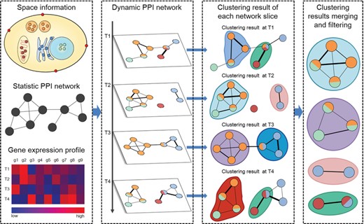
The flowchart of identifying protein complexes from dynamic PPI networks. First, using gene expression profiles and subcellular location data to project the static PPI network as different network slices to construct the dynamic PPI network. In each network slice, proteins are expressed at the same time point, and only the proteins in the same subcellular location can interact with each other. Second, clustering methods are performed on each network slice to generate clusters. Finally, merging or filtering highly overlapping clusters to form protein complexes.
PPI networks
PPI networks are constructed from PPI data sets by denoting proteins as nodes and PPIs as edges. Typically, PPI networks are static, assuming every PPI is constant in any cell and condition. However, PPIs are dynamic inside cells, and their occurrences depend on spatial, temporal and/or contextual variation. Therefore, it is more reasonable to model PPI networks as dynamic systems [71]. Besides, as more and more PPI data from different species are available, constructing interolog PPI networks becomes a new trend to transfer biological knowledge across species [72].
Static PPI networks
Usually, static PPI networks are modeled as simple undirected graphs. For preserving the raw information of PPI determination experiments, several studies represent static PPI network as a bipartite graph, where one part of nodes corresponds to bait proteins and the other part corresponds to prey proteins [39, 73, 74]. Because network weights are crucial for protein complex identification [70], different kinds of biological data have been used to assign weights to PPI networks.
First, TAP-MS data are important information source to calculate PPI affinity scores. Different techniques derive scores that quantify the likelihood of two proteins being observed together by using different procedures and adopt these scores as the weights of edges in PPI networks [75].
Second, topological structure information is widely used to quantify the closeness between node pairs in PPI networks. On this aspect, several methods measure the closeness between two connected nodes based on their common neighbors and degrees [38, 76–78]. Later, NEOComplex [53] further accounts the common neighbors of common neighbors for defining the closeness score of two connected nodes. To improve the reliability of weights, AdjustCD [79] and PE-measure [30] are defined in an iterative manner. Because PPI networks are noisy and incomplete, Chen et al. [80] adapt networks by removing edges with low FS-weight that measuring the overlap degree of the neighborhoods of two nodes and introduce edges for indirectly connected nodes with high FS-weight.
Third, Gene Ontology (GO) [81, 82] is commonly used for evaluating PPI reliability. During the past decades, various semantic similarity measures of GO terms have been defined [83] and assigned as the weights of edges in PPI networks. Gene expression data are also widely used for assigning weights to edges in PPI networks. For example, Luo et al. [84] adopt the Pearson correlation coefficient (PCC) of the coding genes of proteins as the weight of an edge. SGNMF [41] assigns the ‘signs’ for edges based on the PCCs of genes, whereas DSMP [85] calculates the distances between gene expression profiles as weights of edges. Besides, ProRank [86] computes the protein sequence similarity score for PPIs as their weights.
Finally, integrating multiple biological data will lead to more accurate weights. In this regard, several approaches combine PPI reliability scores derived from different experimental evidences by different means [87, 88]. Other methods combine topology-based weights with other scores, such as GO similarity score [33, 89, 90] and PCCs of gene expression data [26].
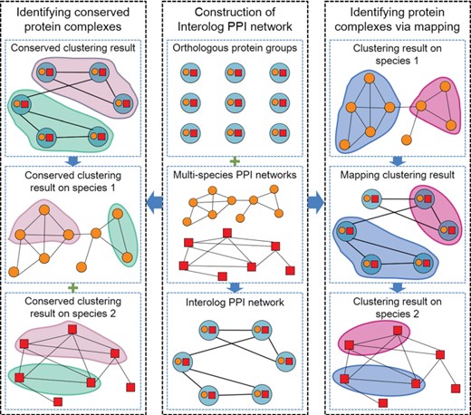
The flowchart of identifying protein complexes from interolog PPI networks. First, the interolog PPI network is constructed by aligning multiple species’ PPI networks. Then, the conserved protein complexes are identified by directly clustering the interolog PPI network. In addition, the orthology protein complex groups are identified by projecting the predicted protein complexes from the source species to other species via the interolog PPI network.
Dynamic PPI networks
In order to capture the dynamic characteristics of PPIs in vivo, a number of studies construct dynamic PPI networks by mapping additional biological information into large-scale PPI data sets [91, 92]. Generally, dynamic PPI networks contain a series of network slices, each consisting of proteins expressed under a condition or at a time point and the corresponding PPIs [92].
Gene expression data are widely used for dynamic PPI network construction. In order to determine expressed proteins or co-expression protein pairs, several methods compare the expression level of proteins with different thresholds [92]. For reducing the impact of inherent background noise in gene expression data, DPPN [52] assigns the active probability at each time point for each protein according to the three-sigma principle [28]. The dynamic PPI networks aforementioned ignore the connections among network slices. To solve this problem, TS-OCD [34] distinguishes stable PPIs and transient PPIs to construct dynamic PPI networks. Stable PPIs are reserved in all network slices, while transient interactions only present in certain time point. Because PPIs also depend on protein subcellular location, several methods constructs more refined dynamic PPI networks by combining protein subcellular information with gene expression data [32, 46]. Other than groups PPIs by time or condition, several methods [55, 93] constructs dynamic PPI networks where each network slice consists of proteins with similar functions and the corresponding PPIs.
Figure 1 shows the general process of identifying protein complexes from dynamic PPI networks. The strategy of identifying protein complexes from dynamic PPI networks is clustering each network slice first and then merges or filters clusters from different network slices based on certain criteria.
Interolog PPI networks
PPIs and protein complexes are frequently conserved in evolution [94]. In order to accurately identify conserved protein complexes and transfer biology information across species, different interolog PPI networks have been developed.
In interolog PPI networks, nodes represent groups of similar proteins, each of which comes from a species, and edges represent conserved PPIs. To determine which proteins are similar and assign edges for which node pairs, various approaches have been developed. The simplest way is assuming every two proteins of different species are similar and linking every two nodes by an edge [95]. A more refined approach is assigning nodes for sequence-similar protein pairs and linking two nodes only if at least one species’ protein pair interacts; meanwhile, the other species’ protein pair share a common interaction partner [96]. In order to control the size of interolog PPI networks, CAPPI [97] groups proteins into families and then assigns a node for each family. The approaches aforementioned ignore the information of interaction partners when determining similarity relationship among proteins. In this regard, IsoRank [72] combines the protein sequences alignment scores and their PPI network neighbor match scores to determine similar protein groups. Since many conserved cellular mechanisms across species cannot be revealed only by protein sequence similarity, COCIN [98] combines domain conservation information with sequence similarity for computing functional similar protein groups.
Figure 2 illustrates the general process of identifying protein complexes from interolog PPI networks. There are two strategies to identify protein complexes from interolog PPI networks. The first strategy directly clusters the interolog PPI network and maps the clustering results to each species. The other strategy clusters the PPI network of a selected species, first, and then maps the identified results into other species via the interolog PPI network.
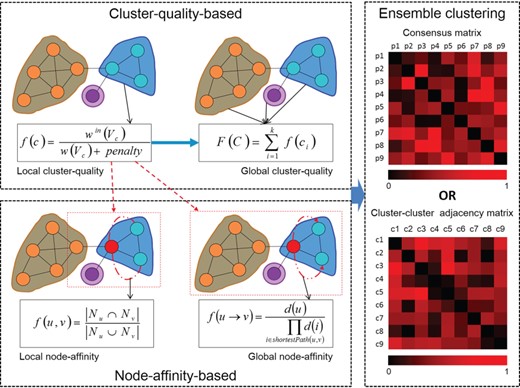
The schematic of computational methods for protein complex identification. Cluster-quality-based methods and node-affinity-based methods measure protein complexes from different aspect, and ensemble clustering methods are developed based on the former two categories of methods.
Methods
Computational methods detect meaningful clusters from PPI networks as protein complexes. According to their methodologies, these methods can be organized into three categories, including cluster-quality-based methods, node-affinity-based methods and ensemble clustering methods. Cluster-quality-based methods treat clusters as measure units; node-affinity-based methods measure the affinity between nodes inside clusters. However, the two categories are not completely disconnected. Actually, some node-affinity-based methods select subgraphs with high cluster-quality as seeds to construct clusters. Finally, ensemble clustering methods combine the outputted clusters of different methods to mine final complexes. Figure 3 shows the schematic and relations of those categories of protein complex identification methods. It should be noticed that each clustering method can be applied to all of the three types of PPI networks to predict protein complexes, as long as it is combined with the corresponding protein complex identifying strategy of each type of network as discussed in the former section.
Cluster-quality-based methods
Cluster-quality-based methods define cluster quality functions and design corresponding algorithms to extract clusters from PPI networks. According to their measuring object, cluster quality functions can be further divided into local-cluster-quality functions and global-cluster-quality functions. Local-cluster-quality functions measure individual clusters, while Global-cluster-quality functions measure all clusters by considering them as a whole.
Local-cluster-quality-based methods
Local-cluster-quality-based methods identify individual clusters with optimal local-cluster-quality in a seed growth manner. Clusters are grown from different seeds via iteratively adding or removing nodes.
Because many protein complexes show dense structures in PPI networks [1], several studies directly employ graph density as the local-cluster-quality function of individual clusters. Starting from a randomly connected node set, Spirin et al. [1] maximize the density of a cluster by ‘moving’ nodes into or out from the cluster according to the Metropolis criteria. Finally, statistically insignificant nodes are removed from clusters, and overlapping clusters are merged if their union remains dense. NCMine [51], Core&Peel [49] and TP-WDPIN [45] identify clusters with density larger than a threshold value. NCMine [51] grows a cluster from each node by adding neighbors according to degree centrality order. During addition, the density change of the cluster must be less than a threshold. Finally, highly overlapping clusters are merged if their union remains dense. Core&Peel [49] extracts clusters from the closed neighborhood of each node based on the degree and core number of nodes. TP-WDPIN [45] selects high-topology potential nodes as seeds. The algorithm first extracts cores from the closed neighborhoods of seeds and then generates a cluster from each core by adding all neighbors that increase the density of the core. After generating all clusters, both Core&Peel [49] and TP-WDPIN [45] discard clusters that are completely contained by others. In order to take advantage of edge weights, DME [99] enumerates all local maximum subgraphs with weighted density exceeding a certain threshold as clusters. NEOComplex [53] expands clusters from each node by recursively adding the neighbor with highest weight of edge connected to the newly added node, until the weighted density of the cluster falls below a threshold. Finally, the algorithm discards highly overlapping clusters and all those with sizes of less than three.
In general, a cluster is considered as a network region with internal connections denser than external connections [100], and many quantitative definitions of this property have been proposed. For example, Chen et al. [101] define the quantitative definition of a cluster based on the in-degree and out-degree of nodes inside the cluster and adapt the GN algorithm [102] to generate clusters. miPALM [77] defines the parametric local modularity of individual clusters. Clusters with maximum parametric local modularity are grown from three-node cliques in a greedy way. Finally, miPALM merges highly overlapping clusters and discards sparse clusters. Cho et al. [103, 104] define the entropy for each cluster. Clusters with minimal graph entropy are generated from the closed neighborhood of each node. Since PPI networks often contain many false-positive edges, methods such as HC-PIN [105], LF-PIN [106] and ClusterONE [70] incorporate weights of edges into cluster quantitative definitions. HC-PIN [105] defines the quantitative definition of a cluster based on the weighted in-degree and out-degree of nodes. The algorithm expands singleton clusters by greedily adding edges according to the clustering value order of edges. Finally, all small clusters are discarded. LF-PIN [106] defines the local fitness of a cluster by multiplying the HC-PIN quantitative definition and the density of the cluster. By iteratively selecting the unclustered edge with highest weight as seeds, clusters with maximal local fitness are constructed by adding or removing nodes via a greedy procedure. ClusterONE [70] defines the cohesiveness score of a cluster based on the cluster size and the intra- and extra-cluster weighted degrees of nodes. The algorithm iteratively selects the unclustered node with highest degree as the seed of a cluster. Clusters with maximal cohesiveness score are constructed by greedily adding or removing nodes. Finally, ClusterONE merges highly overlapping clusters and discards all small and sparse clusters. Later, several improved methods have been proposed. PCE-FR [44] detects pseudocliques based on the fuzzy relation between nodes as seeds of clusters; Zhang et al. [43] redefine the cohesiveness score of a cluster based on the number of triangles related to the cluster; EPOF [107] removes the penalty term from the dominator of the cohesiveness score function.
Because PPI data are imperfect, several methods [73, 95, 96, 108] quantify the likelihood ratio score that a subgraph of the PPI network being a protein complex based on different probability models. The first three methods define different types of seeds and generate individual clusters with maximum likelihood ratio score by adding or removing nodes via a greedy procedure. The last method selects each node as a seed and constructs maximal likelihood ratio score clusters by employing the simulated annealing search.
Global-cluster-quality-based methods
Global-cluster-quality-based methods search for an optimal clustering result with best global-cluster-quality function value. In order to obtain a set of dense clusters, RNSC [109] defines a naive and a scaled cost function for the clustering result. The algorithm first minimizes the naive cost and then the scaled cost of the clustering result by moving nodes between clusters via a restricted procedure. Finally, all small, sparse and weak functional homogeneity clusters are removed. MAE-FMD [33] searches for the clustering result with maximum modularity [110] by applying evolutionary operators on different clustering results. Finally, the algorithm merges functionally similar clusters and discards all singleton and sparse clusters. LCMA [111] considers maximum cliques as initial clusters and iteratively merges highly overlapping clusters until the average density of all clusters is less than a parameter. Ramadan et al. [50] define the fitness value of a clustering result based on the density of individual clusters and apply a genetic algorithm to search the clustering result with maximum fitness value. GS [112, 113] defines the graph description length of a clustering result and searches for the clustering result with minimal description length by merging clusters in a greedy manner.
The aforementioned methods are unable to detect clusters containing peripheral proteins. Therefore, several generative network models, such as RSGNM [114], GMFTP [37] and SGNMF [41], have been proposed. These models generate real PPI networks based on a set of propensity parameters that represent how likely a protein belongs to a protein complex. For identifying clusters, the probability of generating real PPI networks is optimized by tuning propensity parameters. RSGNM [114] generates the PPI network according to Poisson distribution and uses the Laplacian regularizer to smooth estimators of propensity parameters. To mitigate the effects of false-positive PPI noise, GMFTP [37] maximizes the joint probability of generating a real PPI network and protein function profiles. In GMFTP, the PPI network and protein function profiles are generated according to Bernoulli distribution. Ou-Yang et al. [47] maximize the joint probability of generating the PPI network and the domain–domain interaction (DDI) network, where the propensity parameters obey the Bernoulli distribution. SGNMF [41] incorporates a Laplacian regularizer into the Kullback–Leibler divergence between the generated network and the real PPI network.
Since some protein complexes do not show dense structures in PPI networks, Wang and Qian [36] identified clusters whose member nodes have similar neighbors. They define the conductance of a clustering result based on the two-hop transition probability between nodes and then propose two algorithms, SLCP2 and GLSP2, to search the minimum conductance clustering result. SLCP2 is a spectral approximate algorithm for identifying non-overlapping clusters, while GLSP2 is a bottom-up greedy strategy-based algorithm and can identify overlapping clusters.
In order to measure clustering results more comprehensively, several methods combine different global-cluster-quality functions to define a unified function. For example, PPSampler [27] defines the unified function of a clustering result as the negative sum of three different score functions. The algorithm searches the clustering result with minimum unified function score by using a Markov chain Monte Carlo method. Later, PPSampler2 [29] alters the distribution of the three score functions; PPSampler2-PIME [40] adds a regularizer of exclusive PPIs into the unified function of PPSampler2.
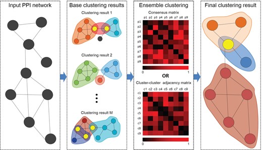
The flowchart of ensemble clustering methods. The base clusters are generated by applying different methods on the PPI network first, and then they are fused to construct a consensus matrix or a cluster-cluster adjacency matrix. Finally, protein complexes are identified from the consensus matrix or the cluster–cluster adjacency matrix.
Node-affinity-based methods
Cluster-quality-based methods ignore the inherent relationship among nodes when identifying clusters. To overcome this problem, node-affinity-based methods have been proposed. Node-affinity-based methods usually generate clusters from seeds by expanding neighbors with high-affinity scores. Based on the measuring scope, node-affinity functions can be further divided into local-node-affinity functions and global-node-affinity functions. Local-node-affinity functions measure the local neighborhood affinity between nodes, while global-node-affinity functions measure the global network affinity between nodes.
The summary of available web servers, stand-alone tools and source code for protein complex identification
| Method | Categorya | Year | Website |
|---|---|---|---|
| ClusterONE [70] | LQ | 2012 | http://www.paccanarolab.org/cluster-one |
| Core&Peel [49] | LQ | 2016 | http://bioalgo.iit.cnr.it/index.php?pg=ppin |
| NCmine [51] | LQ | 2016 | http://apps.cytoscape.org/apps/ncmine |
| RNSC [109] | GQ | 2004 | http://www.cs.toronto.edu/~juris/data/rnsc |
| RSGNM [114] | GQ | 2012 | https://github.com/Zhangxf-ccnu/RSGNM |
| SGNMF [41] | GQ | 2015 | https://github.com/hongyusu/SGNMF |
| MCODE [115] | LA | 2003 | http://apps.cytoscape.org/apps/mcode |
| CFinder [117] | LA | 2006 | http://www.cfinder.org |
| DPClus [76] | LA | 2006 | http://kanaya.naist.jp/DPClus |
| SPICi [119] | LA | 2010 | http://compbio.cs.princeton.edu/spici |
| CMC [79] | LA | 2009 | http://www.comp.nus.edu.sg/~wongls/projects/complexprediction/CMC-26may09 |
| CORE [122] | LA | 2009 | http://i.cs.hku.hk/~alse/hkubrg/projects/core |
| PEWCC [30] | LA | 2013 | http://faculty.uaeu.ac.ae/nzaki/Research.htm |
| ProRank+ [57] | LA | 2014 | http://faculty.uaeu.ac.ae/nzaki/Research.htm |
| MCL [127, 128] | GA | 2000 | https://micans.org/mcl |
| RRW [133] | GA | 2009 | http://imi.kyushu-u.ac.jp/~om |
| NWE [134] | GA | 2010 | http://imi.kyushu-u.ac.jp/~om |
‘LQ’ represents the local-cluster-quality-based methods, ‘GQ’ represents the global-cluster-quality-based methods, ‘LA’ represents the Local-node-affinity-based methods and ‘GA’ represents the global-node-affinity methods.
Local-node-affinity-based methods
To detect dense clusters, MCODE [115] and SWEMODE [116] quantify local-node-affinity based on node weight. MCODE [115] assigns weight to each node based on the highest k-core that contains the node. Clusters are generated by iteratively taking the unseen highest weight node as the seed and then recursively adding unseen neighbors. When all clusters have been generated, the algorithm further processes them by the ‘fluff’ and ‘haircut’ operation. Later, SWEMODE [116] proposes two different schemes to assign weights to nodes. Some methods quantify local-node-affinity based on the number of edges among nodes. For example, Spirin et al. [1] suggest that nodes inside a cluster should completely link to each other and enumerate all maximum cliques in the PPI network as clusters. CFinder [117], DPClus [76] and ICPA [118] assume that the intra-cluster degree of each node should be larger than a threshold value. CFinder [117] sets the threshold to be a constant value and identifies k-clique communities as clusters. DPClus [76] sets the threshold of a cluster based on the density and size of the cluster. The algorithm generates a cluster by selecting the node with the highest weighted degree as the seed and then adding neighbors according to node priorities. During expanding, the density of the cluster must be higher than a threshold. When a cluster cannot be further expanded, it is removed from the network for generating the next cluster. IPCA [118] sets the threshold of a cluster based on the size of the cluster. The algorithm constructs clusters in a procedure similar as that of DPClus [76] but ensures the diameter of a cluster is less than a threshold during expanding. Furthermore, nodes would not be removed from the network after a cluster is generated. SPICi [119], OIIP [89] and MKE [35] suggest that the intra-cluster weighted degree of each node should be larger than a threshold. SPICi [119] defines the threshold based on the weighted density and size of the cluster and generates clusters in a procedure similar to that of DPClus [76]. OIIP [89] defines the threshold based on the total edge weights inside the cluster and generates clusters in a procedure similar to that of ICPA [118]. MKE [35] defines the threshold based on the edge weights of the closed neighborhood of the cluster. The algorithm generates clusters by taking high degree nodes as seeds and then iteratively adding weighted best neighbors. CMC [79] suggests that the connectivity between nodes inside a cluster should be larger than a threshold. The algorithm mines all maximal cliques in the PPI network as initial clusters and then ranks them in decreasing weighted density order. Finally, for every highly overlapping clique pair, CMC either discards the one with lower weighted density or merges them into one clique according to the interconnectivity score between them. SCAN [120] assumes that two nodes inside a cluster should share many common neighbors. The algorithm defines the structural similarity for connected node pairs and generates clusters by selecting core nodes as seeds and then recursively including structure-reachable nodes.
Because many real protein complexes exhibit the core attachment architecture [8], some algorithms first detect dense regions in PPI networks as cores and then integrate attachment nodes with each core to form clusters. For example, Pu et al. [121] adopt the non-overlapping clusters outputted by existing methods as cores and take neighbors connected with sufficient fraction of a core as the attachment nodes of that core. CORE [122], COACH [123] and PEWCC [30] take neighbors that connected with more than half of the nodes of a core as the attachment nodes of that core. CORE [122] identifies cores based on the probability of two nodes forming a protein complex core; COACH [123] identifies dense cores from the closed neighborhood of each node by using the core removal algorithm; PEWCC [30] identifies cores with weighted clustering coefficient larger than a threshold by using a procedure similar to that of COACH [123]. DCU [38] identifies high expected density cores from the closed neighborhood of each node via a greedy procedure. The algorithm selects neighbors with relative degree inside a core larger than a threshold as the attachment nodes of that core. WPNCA [42] extracts cores with high weighted density from dense preliminary clusters. For each core, its attachment nodes are selected from the preliminary cluster containing it.
Different from previous conclusions, Chen et al. [124] discover that most protein complexes are sparse in PPI networks. They identify starlike clusters by taking high degree nodes as seeds and then adding neighbors via a random procedure. ProRank [86] and ProRank+ [57] apply the spoke model to generate clusters based on node types and importance values and then merge highly overlapping clusters by different procedures. Dutkowski et al. [97] assume that nodes connected by high weighted edges are likely to form a cluster. They compute edge weights by using a PPI network evolution model, and then remove all low weight edges from the PPI network. After that, each connected component of the remaining network is outputted as a cluster.
Combining additional biological data will predict more biological meaningful clusters. For example, CSO [31] integrates the GO slims [81, 82] of proteins and the core attachment architecture to identify clusters. SPIC [125] splits clusters generated by existing methods into smaller and more refined ones by eliminating mutually exclusive PPIs. Ozawa et al. [126] discard clusters according to DDIs.
Global-node-affinity-based methods
In order to identify dense clusters, several methods such as MCL [127, 128], R-MCL [129], SR-MCL [130] and STM [131] simulate flows inside PPI networks. MCL [127, 128] alternately performs the expansion and inflation operator to the stochastic matrix of a PPI network. The expansion operator simulates flow through nodes, and the inflation operator is responsible for strengthening intra-cluster currents, meanwhile weakening inter-cluster currents. When the stochastic matrix became doubly idempotent, each attractor system in it is outputted as a cluster. To minimize the number of unreasonable size clusters, R-MCL [129] replaces the expansion operator with the ‘Regularize’ operator. In order to identify overlapping clusters, SR-MCL [130] modifies the ‘Regularize’ operator. The algorithm is iteratively re-executed via decreasing the flow to attractor nodes of previous iterations to generate different clustering results. Cho et al. [132] propagate information from an informative node to every other node in the PPI network through every possible path and take each informative node with its information coverage as a cluster. Finally, strong interconnection clusters are merged in a greedy manner. STM [131] propagates signal between every node pair based on the Erlang distribution and then generates clusters based on the signal value received among nodes. Other methods such as RRW [133], NWE [134] and RWRB [39] identify clusters based on random walks with restart. RRW [133] assumes that nodes inside a cluster have equal impact on determining new nodes of the cluster. By selecting high nodes as seeds, the algorithm expands clusters with restricted size in a greedy manner. NWE [134] argues that the nodes with different weight should have different impact on determining new nodes of a cluster. RWRB [39] incorporates the protein bait–prey relationship from TAP-MS data onto the random walk with restart and generates clusters in a procedure similar to that of MCL [127, 128].
Ensemble clustering methods
Figure 4 shows the general process of how ensemble clustering methods identify protein complexes from PPI networks. Each computational method has its unique advantages and shortcomings. Therefore, ensemble clustering methods are proposed to overcome the bias of different methods and generate more accurate clusters. According to their fusing strategies, ensemble clustering methods can be divided into consensus methods and meta-clustering methods.
Consensus methods fuse base clusters by different approa-ches to construct a consensus matrix and then identify final complexes from it. In the consensus matrix, each entry indicates the co-clustered strength of two proteins. Asur et al. [135] calculate the co-clustered strength of two proteins based on the reliability score of base clusters containing the two proteins. TINCD [48] constructs the final consensus matrix by fusing the TAP data based co-complex score matrix and consensus matrices of different PPI networks and proposes a new algorithm to identify final clusters. EnsemHC [54] also combines the co-complex scores that were derived from TAP-MS experiments [75] and the co-clustered strength of pairs of proteins to define a co-cluster matrix for each base clustering result. The consensus matrix is then constructed by fusing co-cluster matrices via an iterative procedure. Friedel et al. [136] define the co-clustered strength of a protein pair as the proportion of Bootstrap sample PPI networks where they are clustered together.
Meta-clustering methods further cluster base clustering results by considering each base cluster as a unit. Greene et al. [137] represent base clustering results into a complete weighted graph, where nodes represents base clusters and the weights of edges are assigned as the [0, 1]-normalized Pearson correlation between base clusters. By considering each node as a meta-cluster, they iteratively merge meta-clusters in a greedy manner to construct a hierarchical tree and then remove all unstable subtrees from the hierarchical tree.
Evaluation
In this section, we comprehensively evaluate the performance of different computational methods on two widely used benchmark PPI datasets, that is, the DIP dataset [58] and the Collins dataset [138].
Evaluation metrics
Seven metrics are commonly used for evaluating protein complex identification methods, including Precision, Recall, F-measure, Sensitivity (Sn), Positive Predictive Value (PPV), Accuracy (Acc), and Proportion of Significant Complexes (PSC).
In Equation (6), |${N}_i$| is the size of the ith reference protein complex.
Performance comparison of 17 computational methods using CYC2008 as reference protein complex set
| Categorya | Methodb, c | # predicted complexes | Precision | Recall | F-measure | Sn | PPV | ACC |
|---|---|---|---|---|---|---|---|---|
| (a) DIP dataset | ||||||||
| LQ | ClusterONE [70] | 361 | 0.421 | 0.353 | 0.384 | 0.398 | 0.664 | 0.514 |
| Core&Peel [49] | 788 | 0.456 | 0.466 | 0.461 | 0.461 | 0.553 | 0.505 | |
| NCMine [51] | 1520 | 0.318 | 0.510 | 0.392 | 0.517 | 0.397 | 0.453 | |
| GQ | RNSC [109] | 238 | 0.555 | 0.382 | 0.453 | 0.406 | 0.666 | 0.520 |
| RSGNM [114] | 560 | 0.332 | 0.480 | 0.393 | 0.538 | 0.554 | 0.546 | |
| SGNMF [41] | 686 | 0.310 | 0.566 | 0.401 | 0.594 | 0.580 | 0.587 | |
| LA | MCODE [115] | 137 | 0.628 | 0.252 | 0.360 | 0.306 | 0.632 | 0.440 |
| CFinder [117] | 133 | 0.632 | 0.245 | 0.353 | 0.482 | 0.376 | 0.425 | |
| DPClus [76] | 322 | 0.494 | 0.426 | 0.458 | 0.467 | 0.580 | 0.521 | |
| SPICi [119] | 325 | 0.360 | 0.353 | 0.356 | 0.499 | 0.523 | 0.511 | |
| CMC [79] | 560 | 0.527 | 0.517 | 0.522 | 0.591 | 0.515 | 0.552 | |
| CORE [122] | 1644 | 0.155 | 0.630 | 0.249 | 0.597 | 0.497 | 0.545 | |
| PEWCC [30] | 1282 | 0.500 | 0.574 | 0.534 | 0.595 | 0.493 | 0.542 | |
| ProRank+ [57] | 433 | 0.270 | 0.262 | 0.266 | 0.355 | 0.482 | 0.414 | |
| GA | MCL [127, 128] | 1570 | 0.199 | 0.708 | 0.311 | 0.516 | 0.705 | 0.603 |
| RRW [133] | 384 | 0.466 | 0.424 | 0.444 | 0.460 | 0.492 | 0.476 | |
| NWE [134] | 365 | 0.493 | 0.421 | 0.455 | 0.435 | 0.594 | 0.508 | |
| (b) Collins dataset | ||||||||
| LQ | ClusterONE [70] | 323 | 0.625 | 0.569 | 0.596 | 0.658 | 0.625 | 0.642 |
| Core&Peel [49] | 407 | 0.526 | 0.370 | 0.434 | 0.509 | 0.600 | 0.553 | |
| NCMine [51] | 822 | 0.691 | 0.385 | 0.494 | 0.568 | 0.557 | 0.563 | |
| GQ | RNSC [109] | 352 | 0.565 | 0.564 | 0.565 | 0.602 | 0.732 | 0.664 |
| RSGNM [114] | 283 | 0.555 | 0.468 | 0.508 | 0.579 | 0.602 | 0.590 | |
| SGNMF [41] | 290 | 0.666 | 0.485 | 0.561 | 0.564 | 0.633 | 0.598 | |
| LA | MCODE [115] | 142 | 0.746 | 0.331 | 0.459 | 0.586 | 0.515 | 0.549 |
| CFinder [117] | 114 | 0.789 | 0.272 | 0.405 | 0.569 | 0.492 | 0.529 | |
| DPClus [76] | 314 | 0.615 | 0.559 | 0.585 | 0.620 | 0.680 | 0.649 | |
| SPICi [119] | 130 | 0.815 | 0.355 | 0.495 | 0.542 | 0.643 | 0.590 | |
| CMC [79] | 225 | 0.800 | 0.333 | 0.471 | 0.550 | 0.579 | 0.565 | |
| CORE [122] | 384 | 0.539 | 0.566 | 0.552 | 0.622 | 0.658 | 0.640 | |
| PEWCC [30] | 589 | 0.788 | 0.306 | 0.441 | 0.507 | 0.586 | 0.545 | |
| ProRank+ [57] | 659 | 0.717 | 0.363 | 0.482 | 0.577 | 0.485 | 0.529 | |
| GA | MCL [127, 128] | 272 | 0.640 | 0.547 | 0.589 | 0.677 | 0.641 | 0.659 |
| RRW [133] | 278 | 0.540 | 0.441 | 0.485 | 0.494 | 0.694 | 0.586 | |
| NWE [134] | 527 | 0.507 | 0.630 | 0.562 | 0.589 | 0.708 | 0.645 | |
aSee the footnote of Table 3.
bAll methods are rerun by us. The predicted result of each method is obtained by tuning its parameters to maximize F-measure, and the optimized parameter values are given in Table S1 in Supporting Information S1.
cThe best performance is highlighted with bold font, the performance ranked second is highlighted with underline and the performance ranked third is highlighted with italic in each column.
Performance comparison
We compare the performance of 17 state-of-the-art computational methods: ClusterONE [70], Core&Peel [49] and NCmine [51] are local-cluster-quality-based methods; RNSC [109], RSGNM [114] and SGNMF [41] are global-cluster-quality-based methods; MCODE [115], CFinder [117], DPClus [76], SPICi [119], CMC [79], CORE [122], PEWCC [30] and ProRank+ [57] are local-node-affinity-based methods and MCL [127, 128], RRW [133] and NWE [134] are global-node-affinity methods. The reasons for selecting these methods are as follows: (1) they achieved the best performance in this field and (2) the implementations of these methods are available. These methods were evaluated on two widely used benchmark PPI datasets, including the DIP dataset [58] and the Collins dataset [138]. The DIP dataset is constructed based on the latest version of DIP database [58], containing 22 763 PPIs among 5015 yeast proteins. The Collins dataset [138] contains 9074 high-confidence PPIs among 1622 yeast proteins. We rerun the 17 methods (Table 3) on the two benchmark datasets. It is worth noting that the previous reviews [21–25] only evaluated the predictors published in 2010 and before. In this study, 7 of the 17 evaluated methods are proposed after 2010.
Performance comparison of 17 methods on for identifying small and large protein complexes using CYC2008 as reference protein complex set
| Categorya | Methodb,c | Small complexes | Large complexes | |||||||
|---|---|---|---|---|---|---|---|---|---|---|
| # predicted small complexes | Precision | Recall | F-measure | # Predicted large complexes | Precision | Recall | F-measure | |||
| (a) DIP dataset | ||||||||||
| LQ | ClusterONE [70] | 142 | 0.070 | 0.039 | 0.050 | 219 | 0.425 | 0.537 | 0.474 | |
| Core&Peel [49] | 305 | 0.151 | 0.170 | 0.160 | 483 | 0.499 | 0.564 | 0.529 | ||
| NCMine [51] | 317 | 0.129 | 0.131 | 0.130 | 1203 | 0.260 | 0.651 | 0.372 | ||
| GQ | RNSC [109] | 102 | 0.265 | 0.116 | 0.161 | 136 | 0.471 | 0.523 | 0.496 | |
| RSGNM [114] | 131 | 0.153 | 0.077 | 0.103 | 429 | 0.221 | 0.617 | 0.326 | ||
| SGNMF [41] | 211 | 0.094 | 0.081 | 0.087 | 475 | 0.227 | 0.725 | 0.346 | ||
| LA | MCODE [115] | 59 | 0.322 | 0.081 | 0.130 | 78 | 0.603 | 0.383 | 0.468 | |
| CFinder [117] | 0 | – | – | – | 133 | 0.368 | 0.396 | 0.382 | ||
| DPClus [76] | 97 | 0.237 | 0.089 | 0.129 | 225 | 0.378 | 0.611 | 0.467 | ||
| SPICi [119] | 22 | 0.364 | 0.031 | 0.057 | 303 | 0.221 | 0.544 | 0.314 | ||
| CMC [79] | 75 | 0.253 | 0.073 | 0.114 | 485 | 0.396 | 0.711 | 0.509 | ||
| CORE [122] | 1292 | 0.086 | 0.405 | 0.142 | 352 | 0.224 | 0.597 | 0.326 | ||
| PEWCC [30] | 16 | 0.063 | 0.004 | 0.007 | 1266 | 0.352 | 0.745 | 0.478 | ||
| ProRank+ [57] | 259 | 0.085 | 0.085 | 0.085 | 174 | 0.339 | 0.309 | 0.323 | ||
| GA | MCL [127, 128] | 1214 | 0.125 | 0.502 | 0.200 | 356 | 0.199 | 0.530 | 0.290 | |
| RRW [133] | 0 | – | – | – | 384 | 0.294 | 0.658 | 0.407 | ||
| NWE [134] | 218 | 0.206 | 0.174 | 0.189 | 147 | 0.503 | 0.490 | 0.497 | ||
| (b) Collins dataset | ||||||||||
| LQ | ClusterONE [70] | 173 | 0.462 | 0.336 | 0.389 | 150 | 0.527 | 0.631 | 0.574 | |
| Core&Peel [49] | 62 | 0.290 | 0.066 | 0.107 | 345 | 0.441 | 0.644 | 0.523 | ||
| NCMine [51] | 0 | – | – | – | 822 | 0.617 | 0.691 | 0.652 | ||
| GQ | RNSC [109] | 256 | 0.379 | 0.405 | 0.392 | 96 | 0.740 | 0.584 | 0.653 | |
| RSGNM [114] | 40 | 0.275 | 0.058 | 0.096 | 243 | 0.412 | 0.698 | 0.518 | ||
| SGNMF [41] | 65 | 0.246 | 0.073 | 0.113 | 225 | 0.507 | 0.678 | 0.580 | ||
| LA | MCODE [115] | 17 | 0.412 | 0.027 | 0.051 | 125 | 0.632 | 0.604 | 0.618 | |
| CFinder [117] | 43 | 0.349 | 0.062 | 0.105 | 71 | 0.746 | 0.450 | 0.561 | ||
| DPClus [76] | 176 | 0.455 | 0.335 | 0.386 | 138 | 0.572 | 0.644 | 0.606 | ||
| SPICi [119] | 28 | 0.536 | 0.073 | 0.129 | 102 | 0.676 | 0.597 | 0.634 | ||
| CMC [79] | 26 | 0.385 | 0.037 | 0.070 | 199 | 0.729 | 0.611 | 0.665 | ||
| CORE [122] | 265 | 0.366 | 0.413 | 0.388 | 119 | 0.622 | 0.604 | 0.612 | ||
| PEWCC [30] | 0 | – | – | – | 589 | 0.732 | 0.638 | 0.681 | ||
| ProRank+ [57] | 93 | 0.280 | 0.097 | 0.144 | 566 | 0.712 | 0.651 | 0.680 | ||
| GA | MCL [127, 128] | 164 | 0.476 | 0.328 | 0.388 | 108 | 0.639 | 0.624 | 0.631 | |
| RRW [133] | 161 | 0.242 | 0.178 | 0.205 | 117 | 0.624 | 0.591 | 0.607 | ||
| NWE [134] | 440 | 0.327 | 0.541 | 0.408 | 87 | 0.770 | 0.523 | 0.623 | ||
Tables 4 shows the overall performance of the 17 methods in terms of Precision, Recall, F-measure, Sn, PPV and Acc on the two benchmark datasets, respectively. In these experiments, the CYC2008 database [65] is used as the reference protein complexes set, and the match threshold |$\upomega$| is set as 0.2 by following those studies [21, 53, 115]. We mainly focus on Precision, Recall and F-measure because Sn, PPV and Acc have severe limitations [21]. The parameters of each method are optimized based on the F-measure, and the optimized values are given in Table S1 in Supporting Information S1. From these tables, we observe the following phenomena. (i) The performance of most methods on the Collins dataset is better than that on the DIP dataset. The reason is that the DIP dataset contains many noise PPIs. In particular, the high reliable interaction subset of the DIP dataset only contains 5470 PPIs, indicating that more than 75% PPIs in the DIP dataset may be false-positive noise. The performance of CMC [79] and PEWCC [30] is better on the DIP dataset than that on the Collins dataset because they change the PPI network by filtering low reliable edges and introduce new edges between nodes. (ii) All methods show unstable performance on different datasets, indicating they heavily rely on PPI networks. For example, ClusterONE [70] achieves the best F-measure on the Collins dataset, while its performance on the DIP dataset is very poor. The reason is that the DIP dataset lacks PPI weights and contains a large amount of false-positive PPIs. (iii) Local-node-affinity-based methods show state-of-the-art Precision and F-measure, while global-node-affinity-based methods achieve the best Recall.
Performance comparison of 17 computational methods in terms of PSC in biological process, molecular function and cellular component
| Categorya | Methodb,c | # predicted complexes | PSC | ||
|---|---|---|---|---|---|
| BPd | MFd | CCd | |||
| (a) DIP dataset | |||||
| LQ | ClusterONE [70] | 361 | 0.568 | 0.396 | 0.482 |
| Core&Peel [49] | 788 | 0.708 | 0.528 | 0.647 | |
| NCMine [51] | 1520 | 0.634 | 0.502 | 0.568 | |
| GQ | RNSC [109] | 238 | 0.744 | 0.504 | 0.580 |
| RSGNM [114] | 560 | 0.575 | 0.409 | 0.468 | |
| SGNMF [41] | 686 | 0.466 | 0.376 | 0.391 | |
| LA | MCODE [115] | 137 | 0.803 | 0.518 | 0.679 |
| CFinder [117] | 133 | 0.820 | 0.647 | 0.729 | |
| DPClus [76] | 322 | 0.733 | 0.571 | 0.590 | |
| SPICi [119] | 325 | 0.545 | 0.443 | 0.452 | |
| CMC [79] | 560 | 0.857 | 0.720 | 0.752 | |
| CORE [122] | 1644 | 0.159 | 0.119 | 0.128 | |
| PEWCC [30] | 1282 | 0.800 | 0.665 | 0.720 | |
| ProRank+ [57] | 433 | 0.374 | 0.273 | 0.344 | |
| GA | MCL [127, 128] | 1570 | 0.146 | 0.102 | 0.118 |
| RRW [133] | 384 | 0.706 | 0.534 | 0.609 | |
| NWE [134] | 365 | 0.658 | 0.416 | 0.515 | |
| (b) Collins dataset | |||||
| LQ | ClusterONE [70] | 323 | 0.526 | 0.402 | 0.427 |
| Core&Peel [49] | 407 | 0.835 | 0.715 | 0.789 | |
| NCMine [51] | 822 | 0.940 | 0.852 | 0.895 | |
| GQ | RNSC [109] | 352 | 0.386 | 0.259 | 0.324 |
| RSGNM [114] | 283 | 0.777 | 0.664 | 0.731 | |
| SGNMF [41] | 290 | 0.786 | 0.610 | 0.641 | |
| LS | MCODE [115] | 142 | 0.901 | 0.676 | 0.796 |
| CFinder [117] | 114 | 0.842 | 0.544 | 0.702 | |
| DPClus [76] | 314 | 0.506 | 0.379 | 0.427 | |
| SPICi [119] | 130 | 0.923 | 0.715 | 0.777 | |
| CMC [79] | 225 | 0.942 | 0.787 | 0.858 | |
| CORE [122] | 384 | 0.372 | 0.263 | 0.315 | |
| PEWCC [30] | 589 | 0.969 | 0.864 | 0.910 | |
| ProRank+ [57] | 659 | 0.910 | 0.787 | 0.863 | |
| GS | MCL [127, 128] | 272 | 0.772 | 0.581 | 0.566 |
| RRW [133] | 278 | 0.629 | 0.489 | 0.590 | |
| NWE [134] | 527 | 0.245 | 0.167 | 0.201 | |
Both small and large protein complexes are ubiquitous in cells [55]. Here, those complexes composed of two or three proteins are referred as small complexes, and complexes containing more than three proteins are referred as large complexes. In CYC2008, the numbers of small and large protein complexes are 259 and 149, respectively. In order to further evaluate different methods, Table 5 gives the Precision, Recall and F-measure values of each method on small and large protein complexes. From Table 5, it is obvious that small complexes remain difficult to identify. On the Collins dataset, the best F-measure of small complexes is only 0.408, while that of the large complexes is 0.681. Furthermore, global-node-affinity-based methods outperform other methods on identifying small complexes. For identifying large complexes, both local-cluster-affinity-based and local-node-affinity-based methods achieve the state-of-the-art performance. In particular, NEW is the best tool for identifying small complexes, and CMC is the best tool for identifying large complexes. Based on the observations from Tables 4 and 5, we conclude that each method has its own advantages, and integration of different methods will further improve the performance of protein complex identification. In this regard, several ensemble clustering methods such as TINCD [48] and EnsemHC [54] have shown better performance than base methods in terms of Recall and Acc.
Tables 6 shows the overall performance of the 17 methods in terms of PSC on the two benchmark datasets. The P-values with Bonferroni correction for predicted protein complexes are calculated by using the stand-alone tool GO::TermFinder [142], and the significant threshold is set as 0.01 by following this study [21]. In general, the performance for most methods on the Collins dataset is also better than that on the DIP dataset. Methods like ClusterONE [70], RNSC [109] and NWE [134] decrease their minimum size cutoff of protein complexes to 2 on the Collins dataset, leading to lower PSC than that on the DIP dataset because protein complexes with the size of 2 have high P-values [85]. Furthermore, some local-cluster-quality-based methods and local-node-affinity-based methods, such as NCMine [51], MCODE [115], CFinder [117] and PEWCC [30], identify dense and large regions in PPI network as complexes; therefore, they show high PSC.
Furthermore, we give a performance comparison of different predictors on the dynamic PPI networks constructed from the DIP dataset, and the results are shown in Table 7. Compared with Table 4, it is obvious that the predictors on dynamic networks outperform those on static networks. In addition, CPredictor2.0 [55] achieves the best F-measure, indicating that protein function information is highly effective for protein complex identification.
Discussion and conclusion
All the aforementioned methods have greatly promoted the development of protein complex identification. However, the following problems should be addressed for further promoting this important field.
PPI datasets
PPI datasets are critical for protein complex identification. There are two main problems of the existing PPI datasets [145]. (1) The available PPIs are incomplete [11]. For example, the estimated number of non-redundant human PPIs is about 650 000 [146], whereas the number of non-redundant human PPIs collected in the latest version of BioGRID database [59] is only 375 840, indicating the coverage is less than 60%. (2) The PPI data sets contain many false-positives [147–149] caused by experiment conditions, the contaminating nucleic acid used in experiments [150] and technical biases [151]. Table 8 shows the false-positive rate of PPIs in the three PPI databases against the Negatome 2.0 [152] database, including DIP, BioGRID and MINT. Negatome 2.0 contains 6532 non-interacting protein pairs reported in literature or derived from protein complex three-dimensional structures. It shows that the highest false-positive PPI rate of the three PPI databases is 4.33%.
Performance comparison of methods on different dynamic PPI networks constructed from the DIP data set using CYC2008 as reference set
| Networka, b | # predicted complexes | Identifying method | DIP version | Precision | Recall | F-measure | Sn | PPV | ACC |
|---|---|---|---|---|---|---|---|---|---|
| TC-PINs [143] | 2063 | MCL [127, 128] | 10 October 2010 | 0.215 | 0.569 | 0.312 | – | – | – |
| DPINs [28] | 1289 | CPM [144] | 28 February 2012 | 0.328 | 0.507 | 0.399 | – | – | – |
| Zhang et al. [52] | – | Zhang et al. [52] | – | 0.483 | 0.471 | 0.477 | 0.373 | 0.694 | 0.509 |
| ST-APIN [46] | 1761 | MCL [127, 128] | 10 October 2010 | 0.339 | 0.605 | 0.435 | – | – | – |
| WDPIN [45] | 550 | TP-WDPIN [45] | 14 January 2016 | 0.466 | 0.436 | 0.451 | – | – | – |
| CPredictor2.0 [55] | 636a | MCL [127, 128] | 13 February 2017 | 0.552 | 0.542 | 0.547 | 0.397 | 0.711 | 0.531 |
aThe predicted result of CPredictor2.0 is obtained by reruning the method, while the predicted results on other dynamic PPI networks are adopted from the origin papers and then transformed by us.
bThe best performance is highlighted with bold font.
False positive PPI rate of different database against the Negatome 2.0 data set
| Database | # overlapping proteins | # overlapping protein–PPIsa | No. of false-positive PPIs | False-positive PPI rate |
|---|---|---|---|---|
| DIP [58] | 1066 | 4529 | 75 | 01.65% |
| BioGRID [59] | 1944 | 18351 | 794 | 04.33% |
| MINT [61] | 1164 | 15721 | 254 | 01.61% |
| Database | # overlapping proteins | # overlapping protein–PPIsa | No. of false-positive PPIs | False-positive PPI rate |
|---|---|---|---|---|
| DIP [58] | 1066 | 4529 | 75 | 01.65% |
| BioGRID [59] | 1944 | 18351 | 794 | 04.33% |
| MINT [61] | 1164 | 15721 | 254 | 01.61% |
aThese PPIs are nonredundant and consisting of only proteins overlapping with the Negatome 2.0.
In order to obtain complete and reliable PPI datasets, many research groups combine multiple techniques to determine PPIs [153]. This goal also can be achieved by assigning weights to observed interactions based on additional biological data [154], characterizing proteins across cell types and subcellular localizations [155] and aligning PPI networks [156]. Furthermore, PPI network alignment would be benefited from introducing the evolutionary relationship by the protein remote homology detection techniques [157–161]. Link prediction paradigms [162–164], which have been successfully applied in various areas [165, 166], are also potential methods for reconstructing PPI networks.
Dynamic PPI networks
Dynamic PPI networks are the key for further improving the performance of protein complex identification. Since protein function information is highly helpful for identifying protein complexes, new dynamic PPI networks should be constructed based on this kind of information. Recently, researchers point out that a PPI may have different scores in different conditions [167, 168]. Therefore, dynamic PPI networks reflecting this property would be very helpful for promoting protein complex identification. In this regard, Zhang et al. [52] assign dynamic weights to PPIs based on the probabilities that proteins expressing at different time points.
Protein complex identification methods
Most protein complex identification methods tend to identify dense and large regions in PPI networks as protein complexes. However, a large proportion of real protein complexes are small and sparse [55, 124]. In order to further improve the performance, new predictors should be designed to accurately identify not only dense and large protein complexes but also small and sparse ones. To achieve this goal, new predictors can be constructed based on the PPI weights that fuse more kinds of biological information, such as protein sequences [169, 170], disorders regions [171, 172], etc. In addition, the ensemble clustering methods are a new trend to construct more accurate meta-predictors. When developing an accurate meta-predictors, the following aspects should be considered. (1) Many protein complexes can only be predicted by some specific methods. Therefore, the meta-predictors should give these complexes high confidence scores to correctly predict these complexes. (2) Some false complexes would be predicted by multiple base predictors. The meta-predictors should correct these false positives by removing the false proteins from complexes. By deriving protein co-cluster strength from base clustering results [48, 54, 135–137] and by further integrating protein co-complex scores derived from TAP-MS experiments [48, 54], the existing meta-predictors not only reduce the impact of false-positive PPI noise but also add some missing PPI information. Therefore, they achieve better performance than base methods. However, most meta-predictors do not have a scoring system that assigns confidence scores to clusters [48, 54, 136, 137], or the scoring system only considers network topology information [135]. Therefore, they would miss many real protein complexes that can only be predicted by a single base method. Furthermore, all these meta-predictors integrate the predicted results of different base methods in an unsupervised manner. Therefore, false complexes predicted by multiple base methods will still be incorrectly predicted by these meta-predictors. More specifically, these meta-predictors cannot remove false-positive proteins predicted by multiple base methods from predicted complexes. In order to develop more accurate meta-predictors, biological relevant protein complex features should be combined with PPI network-based protein complex features in a supervised manner.
Another problem is that different methods heavily depend on the PPI networks. Since most PPI data sets are incomplete and unreliable, the performance of different methods is limited. In this regard, generative network models [37, 47, 114] are potential solutions, and their performance would be further improved by integrating more information [37, 47]. Furthermore, they can output sparse complexes, even those consist of proteins that are not connected in PPI networks. It is also feasible to assign scores to protein pairs and improve the quality of networks by removing low-reliability edges and introducing edges to protein pairs with high affinity score [30, 79, 88]. Supervised machine learning models, such as Bayesian network models [108], also can be used for identifying protein complexes. However, most of the protein complex features are network topological features, preventing the performance improvement of these models. Therefore, biologically relevant protein complex features should be explored to improve the performance of the supervised models.
With the availability of genomic-scale PPI data for various species, it is important to develop computational methods to accurately and efficiently identify protein complexes from PPI networks.
The databases of PPIs/protein complexes are introduced and discussed.
The three types of PPI networks, including static, dynamic and interolog networks, are introduced, and the strategies of identifying protein complexes from them are described.
The computational methods for identifying protein complexes from PPI networks are introduced, and their advantages and shortcomings are discussed. The existing available web servers and stand-alone tools in this filed are given.
The performance of 17 state-of-the-art computational methods for identifying protein complexes from PPI networks is evaluated and compared on two widely used benchmark datasets. Finally, some challenges and perspectives in this field are discussed.
Acknowledgements
The authors are very much indebted to the three anonymous reviewers, whose constructive comments are very helpful in strengthening the presentation of this article.
Funding
This work was supported by the National Natural Science Foundation of China (61672184, 61732012 and 61822306), the Fok Ying-Tung Education Foundation for Young Teachers in the Higher Education Institutions of China (161063), the Shenzhen Overseas High Level Talents Innovation Foundation (Grant No. KQJSCX20170327161949608), the Guangdong Natural Science Funds for Distinguished Young Scholars (2016A030306008) and the Scientific Research Foundation in Shenzhen (JCYJ20180306172207178).
Zhourun Wu is a PhD candidate at the School of Computer Science and Technology, Harbin Institute of Technology, Shenzhen, Guangdong, China. His research areas include bioinformatics and machine learning.
Qing Liao, PhD, is an associate professor at the School of Computer Science and Technology, Harbin Institute of Technology, Shenzhen, Guangdong, China. Her research areas include bioinformatics and machine learning.
Bin Liu, PhD, is a professor at the School of Computer Science and Technology, Harbin Institute of Technology, Shenzhen, Guangdong 518055, China, and School of Computer Science and Technology, Beijing Institute of Technology, Beijing 100081, China. His expertise is in bioinformatics, nature language processing and machine learning.
