


Abstract
Recent advances in sequencing, mass spectrometry and cytometry technologies have enabled researchers to collect large-scale omics data from the same set of biological samples. The joint analysis of multiple omics offers the opportunity to uncover coordinated cellular processes acting across different omic layers. In this work, we present a thorough comparison of a selection of recent integrative clustering approaches, including Bayesian (BCC and MDI) and matrix factorization approaches (iCluster, moCluster, JIVE and iNMF). Based on simulations, the methods were evaluated on their sensitivity and their ability to recover both the correct number of clusters and the simulated clustering at the common and data-specific levels. Standard non-integrative approaches were also included to quantify the added value of integrative methods. For most matrix factorization methods and one Bayesian approach (BCC), the shared and specific structures were successfully recovered with high and moderate accuracy, respectively. An opposite behavior was observed on non-integrative approaches, i.e. high performances on specific structures only. Finally, we applied the methods on the Cancer Genome Atlas breast cancer data set to check whether results based on experimental data were consistent with those obtained in the simulations.
Introduction
The accumulation of large molecular data sets has fueled the development of translational bioinformatics and systems biology that share a holistic view on omics data. While the former aims to link biological to clinical data to improve our understanding of disease mechanisms, the latter explores the basic functional properties of living organisms based on the premise that biological processes build upon the interplay between macromolecules. Both approaches rely on the idea that biological mechanisms (and, more generally, phenotypic traits) can only be fully captured through the study of molecular interactions among different omics layers.
Multi-omic approaches have received much attention in recent years for their potential applications in clinics. In genome-wide association studies for example, the mechanisms by which the identified loci influence phenotypes remain generally unknown and are likely to be unveiled using functional genomics. Cancer subtype diagnosis, commonly determined by clinicopathologic parameters (i.e. morphological variables), tend to underestimate inter-patient variability by classifying patients with different responses to treatment or long-term prognosis in the same group [1]. By crossing genomic, epigenomic, transcriptomic and proteomic data, the Cancer Genome Atlas (TCGA) network was able to refine breast cancer classes into phenotypically homogeneous groups [2]. Quigley et al. [3] demonstrated that genetic susceptibility in breast cancer is, in some cases, context specific and requires the combination of transcriptomic and epigenomic data to explain the mechanisms of risk alleles. Similarly, Meng et al. [4] showed that the leukemia extravasation signaling pathway could only be identified through the integration of gene and protein expression. These observations show that the integration of multiple sources has the potential to (i) mitigate the risk of false positives when multiple sources of evidence point to the same pathway [5], (ii) lead to novel insights into the molecular crosstalk between omics layers that underlies complex traits and (iii) identify new biomarkers to stratify patients into novel, clinically relevant disease subtypes [6].
The increasing availability of large heterogeneous data sets (e.g. TCGA, the International Cancer Genome Consortium and the Asian Cancer Research Group) has prompted the development of novel integrative methods that aim to capture weak yet consistent patterns across data types. This task is, however, non-trivial due to (i) the increased dimensionality that makes inference weaker, (ii) the challenge to decipher data-specific from inter-source variations and (iii) the different types of noise and confounding effects across platforms, resulting in data heterogeneity. For example, next-generation sequencing (NGS) and microarray data are commonly modeled with negative binomial and Gaussian distributions, respectively.
Despite these challenges, at least five major strategies have been proposed to integrate heterogeneous omics data. The first strategy, conceptual integration, consists of analyzing each omics separately and combining the results at the interpretation step. Because of its simplicity and the lack of gold standard in the domain, this type of integration has been largely applied in multi-omic analysis [7]. One obvious drawback of such method is its limited power to uncover modest but coordinated variations acting at different biological layers [8]. The 2nd strategy, consensus clustering, generates an overall sample classification after an initial clustering step performed in each omics. Although successfully applied in TCGA to refine breast cancer subtypes [2], this two-step procedure of separate clusterings followed by post hoc integration limits the power to detect crosstalk between omics. The 3rd strategy, concatenation-based integration, allows the application of standard machine learning techniques after concatenation of omics measurements into a single matrix. While such strategy turned out to have high discriminative power in supervised framework [9], it is sensitive to the data size when applied naively and consequently returns results biased toward the omics with the most numerous features. However, recent supervised concatenation approaches account for unbalanced data sizes [10]. Additionally, concatenation-based integration does not account for relationships across sources and heterogeneous measurement error across platforms. The 4th strategy searches for common variations across omics using matrix factorization, Bayesian and network-based approaches specifically tailored for data integration. The 5th strategy, multi-omic pathway enrichment, aims to find pathways that correlate with a particular phenotypic end point, based on their multi-omic profiles. In practice though, the current tools perform pathway enrichment in each omics before combining the obtained P-values [11, 12], similarly to the conceptual integration.
Most of the effort in the area have been concentrated on the 4th strategy where many methods propose to find a joint cluster structure, from which patient stratification and molecular mechanisms can be deduced. The methodological aspects underlying integrative approaches have been recently reviewed [13–16] and led to a classification according to two criteria; whether or not the method under consideration relies on (i) networks and (ii) Bayesian approaches, the network-free non-Bayesian approaches being based on matrix factorization [17].
Most of these methods have been evaluated individually and occasionally compared against iCluster (presented hereafter). To our knowledge, only one benchmark of five network-based and matrix factorization approaches has been performed so far [18], leaving Bayesian methods aside. The methods were evaluated with their default parameters, except for the best-performing one.
In the present work, we propose a comparison of six popular methods, one being in common with [18], using simulated and real-world data (TCGA). Because we are interested in clustering approaches that do not require any prior biological knowledge and that can be widely applicable, the methods were selected on the basis of their ability to deal with any data type and produce clustering at both molecular and sample levels. Therefore, models tailored for specific omic types [19–21] and network-based approaches focusing on patient stratification [22] or network enrichment [23] were left aside.
The methods assessed in this work fall into two categories, Bayesian approaches that extend the finite Dirichlet mixture model and dimension reduction techniques aiming at identifying shared latent variables. To avoid favoring one category over the other in our study, the simulations were generated using one model from each family. Also, like any clustering problem, the determination of the optimal number of clusters is crucial and needs to be addressed carefully. To do so, all methods propose guidelines (presented in their description hereafter) and, in most cases, include the associated code. Because (i) this step has a large impact on the final clustering, (ii) the code is not systematically available and, (iii) in practice, users often test different number of clusters and validate their choice using orthogonal data [35], we decided to separately evaluate this step of estimation of the number of clusters from the clustering itself. In this latter evaluation of the clustering step, the methods were run using the true (simulated) number of clusters and evaluated on their ability to recover the simulated clustering.
The remainder of the paper is organized as follows: in the first section, we briefly present the methods, the simulation scenarios and the evaluation criteria. In the Results section, we present the relative performances of the methods both on simulated and TCGA data. Finally, in the light of the results, we discuss the choice of methods in multi-omic framework in Discussion and conclusion.
Methods
Methods overview
where |$\textit {W}_k$| is the |$p_k \times q$| loading matrix associated with data set |$k$|, |$\textit {Z}$| is the |$q \times N$| common latent variable matrix and |$\boldsymbol {\varepsilon }_k$| is the |$p_k \times N$| uncorrelated error matrix that follows a multivariate Gaussian distribution |$\mathcal {N}_{p_k}(\textit {0},\boldsymbol {\psi }_k)$| with zero mean and diagonal covariance matrix |$\boldsymbol {\psi }_k = \text {diag}(\sigma _{k,1}^2, \cdots , \sigma _{k,{p_k}}^2)$|. By forcing the latent variables to be equal, iCluster assumes that the |$K$| data sets derive from a set of common factors. Parameter estimation is then performed using an expectation–maximization algorithm on the multivariate normal distribution. The final cluster assignment is determined by k-means clustering on the posterior expectation of the latent factors |$E(\textit {Z}|\textit {X})$|. An |$l_1$| penalty can be imposed on the loading coefficients to perform variable selection. The penalty parameter and the number |$q$| of latent variables are tuned manually using the proportion of deviance (a measure of cluster separability, [25]) from which the number of clusters can be deduced. Indeed, Shen et al. [25] recall that a |$K-1$| rank matrix is sufficient for separating |$K$| clusters. In Shen et al. [24], a cross-validated Rand index (RI) (Clustering performance criteria), measuring the clustering similarity between the training and the test sets, is used for parameter tuning [24]. An extension of the model, iClusterPlus (not evaluated in the present work), allows to account for binary, counts and categorical data.
moCluster also decomposes each data set |$\textit {X}_k$| into a product of shared latent variables |$\textit {Z}$| and a sparse, data-specific, loading matrix |$\textit {W}_k$| [26], similarly to iCluster. The main difference between these two methods is that iCluster derives from factor analysis, whereas moCluster relies on consensus PCA. For this reason, iCluster separates the covariance from the variable-specific variance, allowing heteroscedasticity among omic features. Consensus PCA, on the other hand, assumes that the noise has same variance across variables (|$\sigma _{k,j}^2:=\sigma ^2$|, for all |$j=1,\dots ,p_k$| and |$k=1,\dots ,K$|), making common and unique variations no longer separable [24]. Although this assumption is strong for the analysis of heterogeneous omics, moCluster offers a 100–1000-fold speed increase as compared to iCluster due to its deterministic parameter estimation based on the NIPALS algorithm. A step of soft thresholding may be used for variable selection. To determine the number of latent variables, the authors suggest a visual inspection of the eigenvalues (scree plot) or a permutation test on the same eigenvalues. Similarly, the authors propose to perform a hierarchical clustering on the latent variable matrix to obtain the final clustering, the number of clusters being determined with the gap statistic [27].
where |$\textit {W}^s_k$| of size |$p_k \times q_k$| and |$\textit {Z}^s_k$| of size |$q_k \times N$| are the data-specific loading and latent variable matrices, respectively. Note that |$q$| and |$q_k$| are not necessarily equal, implying that the joint and individual low-rank approximations may be of different dimensions. To guarantee the identifiability of the decomposition, the authors imposed an orthogonality constraint between the joint and individual terms. The parameter estimation is performed by estimating the joint and individual structures iteratively via SVD by fixing one term at a time and minimizing the square norm of the residual matrix for updating the other term. Sparsity is induced during the estimation procedure by an |$l_1$| penalty on the loading matrices. The level of sparsity is determined using the Bayesian information criterion. As with moCluster, the number of joint and individual latent variables is estimated using a permutation approach on the eigenvalues. Unlike iCluster and moCluster that provide tools to cluster samples from the latent variables, Lock and Dunson [35] do not give guideline to generate a final sample clustering.
Again, the authors motivate the addition of data-specific effects by demonstrating that jNMF [31], a similar approach without data-specific term, is more sensitive to random noise and confounding effects. The choice of non-negativity factorization is, on the other hand, motivated by its simple and meaningful interpretation that ‘the whole is an additive linear combination of its parts’ [32]. While non-negative factorization approaches have a naturally sparse and parts-based representation [33], sparsity is nevertheless induced in iNMF by applying an |$l_1$|-penalization on the data-specific term. This constraint imposed on the data-specific effects implies that the parameter |$\lambda$| controls for the factorization homogeneity. The authors also propose to apply an |$l_1$|-penalty on the coefficient matrix |$\textit {W}_k$| to enforce variable selection. The dimension of the shared and specific structures (equal due to the shared coefficient matrix) is chosen through a consensus-based approach that selects the number of latent variables maximizing the clusters stability across multiple iNMF runs. The |$\lambda$| parameter is, on the other hand, determined using an ad hoc procedure that aims to attribute as much of the data as possible to the specific structure while controlling for over-fitting. Unlike the previous approaches, the authors propose a method to perform clustering on the variables, which is out of the scope of this work. Similarly to JIVE, no guidelines are provided to obtain a final sample clustering.
where |$\mathbb{1}$| is the indicator function, |$\phi _{kl}$| controls the association strength between data sets |$k$| and |$l$|, |$c_{ik}$| indicates the cluster allocation of sample |$i$| in data set |$k$| and |$\pi _{c_{ik}k}$| is the mixture proportion associated with cluster |$c_{ik}$| in data set |$k$|. The parameters, including the number of clusters in each source, are inferred via Gibbs sampling. The authors then propose to maximize the posterior expected adjusted Rand index (PEAR) across source-specific clusterings to determine a single global clustering. As pointed out by Wei et al. [14], the model could be extended by modeling the pairwise association at the component level instead of the data set level. Variable selection is not provided by the method, and the maximal number of clusters needs to be fixed by the user. For computational reasons, the authors recommend to set this parameter to half the sample size. However, we noticed that this value led to numerical instabilities and set it to the sample size.
where, for sample |$n$|, |$C_n$| and |$L_{kn}$| are the overall and source-specific cluster allocations in data source |$k$|, |$\alpha _k$| is the adherence of data set |$k$| to the overall clustering and |$q$| is the maximum number of clusters (both shared and source specific). The adherence parameter |$\alpha _k$| models how intertwined specific and shared clusters are. The parameter |$q$| is chosen so that the mean adherence over the sources is maximized, which, according to the authors, results in a small number of selected clusters. Similarly to MDI, a Gibbs sampler is used to estimate the posterior distribution of the parameters.
Data pre-processing
Depending on the model assumptions, the six methods propose different pre-processing steps. Since moCluster and JIVE rely on techniques that treat covariance and variance identically (consensus PCA and SVD), these methods are sensitive to variable scaling. For this reason, data sets are centered or standardized in JIVE and moCluster, respectively. To circumvent the case where ‘the largest data set wins’, data matrices are further weighted by the reverse of their first eigenvalue (moCluster) or their Frobenius norm (JIVE). iNMF also normalizes each matrix by its Frobenius norm after variance stabilization (log transformation) and non-negativity transformation. By contrast, given that iCluster allows heteroscedasticity, only a centering step is performed. At last, no pre-processing is performed with MDI and BCC, considering that Dirichlet mixture models offer enough flexibility. A brief description of the methods, their pre-processing and availability are provided in Table 1.
Description, pre-processing and implementation of the evaluated methods
| Method | Description | Pre-processing | Implementation | |
|---|---|---|---|---|
| Integrative methods | iCluster | Joint latent variable model | Centering | R package iCluster |
| moCluster | Modified consensus PCA | Standardization | R package mogsa | |
| JIVE | Matrix factorization into common and specific variations | Standardization | R package r.jive | |
| iNMF | Joint non-negative matrix factorization | Variance stabilization | Python script | |
| Non-negativity transformation | ||||
| Frobenius normalization | ||||
| MDI | Dirichlet mixture models | None | Matlab script | |
| BCC | Dirichlet mixture models | None | R package bayesCC | |
| Non-integrative methods | GMM | GMMs | None | R package mclust |
| Concatenation | Concatenation and GMMs | None | R package mclust | |
| Consensus clustering | GMMs and maximization of PEAR | None | R packages mclust and mcclust |
Simulation scenarios
The methods presented above were evaluated both on simulated and real data. On simulations, the methods were evaluated on their ability to (i) recover the number of simulated clusters and identify the correct clustering at the (ii) common and (iii) data-specific levels as well as on their (iv) sensitivity. The sensitivity was assessed by varying the level of signal-to-noise ratio (SNR) and the dimension of the shared clusters. Overlaps between the two structures were introduced to assess whether they could hinder the identification of the shared structure. Since the tested methods can roughly be divided in two groups (matrix factorization and Bayesian models), simulations were generated under iNMF (matrix factorization) and BCC (Bayesian model) models to ensure an unbiased evaluation. Each simulation consists of |$K=3$| matrices |$\textit {X}_{k}$| of dimension |$p_k \times N$|, with |$N=60$| samples, and |$p_k$| features in the 3 data matrices with |$P=(180,210,240)$|. Each matrix |$\textit {X}_k$| consists of 3 common clusters made of 20 samples each. Although the number of features is at least one order of magnitude smaller than what is commonly observed in high-throughput omics, they are more amenable to the present large-scale evaluation in terms of runtimes. To evaluate the validity of our results under more realistic settings though, i.e. higher dimension and an important unbalanced number of features, one scenario was also generated with |$P = (300,600,3000)$| features. Details and illustrations of the following simulation scenarios are provided in Supplementary Materials. In addition, the runtimes are provided in Supplementary Table 2.
iNMF-derived scenarios
The first simulation scenarios are derived from iNMF, in which each data matrix |$\textit {X}_k$| is built as the sum of three matrices: one made of three shared diagonal blocks of same dimensions, one with one or two data-specific off-diagonal blocks and one made of random uniform noise. The blocks were constructed by multiplying the binary latent variables (|$\textit {Z}$| and |$\textit {Z}_k$|) with the data-specific loadings |$\textit {W}_k$|. The loadings were simulated under a beta(2,2) distribution, satisfying thus the non-negativity constraint required by iNMF while not diverging too much from a Gaussian distribution (the beta and Gaussian distribution are symmetrical and have a bell shape). The same two levels of noise used in [30] were also used here. This level of noise is controlled by a ‘scattered error’ that replaces either a positive value with zero or a zero with a randomly generated |$(beta(2,2)\times 2)^2$| with a probability |$1-\sigma _s$| dependent of the desired level of noise. A distinctive feature of the simulations in [30] is that the data-specific blocks are aligned with the columns (variables) of the shared structure. In practice, this premise implies that features involved in shared and omic-specific mechanisms are identical. Because probably unrealistic, we simulated specific blocks so they do or do not overlap with the shared structure, where in the first case, the specific blocks randomly overlap with one or two shared block(s). In the context of our study, an overlap between a common and a specific block means that they have some variables in common (Supplementary Figure 1). For both overlap and non-overlap simulations, a given observation belongs to one common cluster and zero to two specific clusters.
Overall, 3 scenarios were generated: iNMF overlap, iNMF non-overlap and iNMF high dimensional, the third being identical to the first apart from the number of features equals to |$p = (300,600,3000)$|. For each combination of scenario and SNR, 100 simulations were generated, adding up to 600 simulations.
BCC-derived scenario
In the same way as the iNMF scenario, the simulation scenario proposed in BCC was extended in two ways: three to five specific clusters adhering loosely to three overall consensus clusters were simulated. Instead of simulating each feature with univariate Gaussian distributions, realizations of |$p_k$|-dimensional Gaussian distributions were generated using the MixSim R package. Unlike iNMF simulations, each observation is uniquely assigned to one specific and one shared cluster. Furthermore, the level of SNR is set by the hypercube parameter in MixSim that controls the space in which the cluster means are sampled. Again, 2 levels of noise were tested, for each of which, 100 simulations were generated, resulting in 200 simulations.
Sensitivity scenario
Methods’ sensitivity was only evaluated on the iNMF scenario by reducing block sizes (both shared and specific). The matrix dimensions were held constant, which implies that samples outside the shared and specific blocks were generated with noise. The number of samples by shared blocks |$n_b$| took values in |$\{5,8,11,14,17,20\}$|. For each combination of noise, overlap (same as in iNMF scenario) and block size, 20 simulations were generated, adding up to a total of 480 simulations.
Clustering performance criteria
The consistency between two clusterings or partitions is commonly measured using the RI [36]. Given |$\textit {c}$| and |$\widehat {c}$| the simulated and estimated clusterings (containing the cluster assignment for each sample), the RI calculation relies on the classification of each sample pair in one of four possible categories. Let |$a$| be the number of sample pairs in the same cluster in |$c$| and |$\widehat {c}$|, |$b$| be the number of pairs in the same cluster in |$c$| but not in |$\widehat {c}$|, |$c$| be the number of pairs in the same cluster in |$\widehat {c}$| but not in |$c$| and |$d$| be the number of pairs in different clusters in |$c$| and |$\widehat {c}$|.
where |$E(RI)$| is the expected RI in case of independence between the two partitions. In the following, the measure of agreement between simulated and estimated clusterings will be presented using the ARI.
From Methods overview we recall that for a given simulation, global and data-specific clusterings are obtained for all methods except iCluster and moCluster for which only a common clustering is available.
Results
In the results presented hereafter, sparsity parameters were left aside, which implies that no penalization was applied in any analysis.
Simulated data
In this section, we evaluate (i) the methods’ ability to recover the correct number of clusters, (ii) the consistency between simulated and estimated clusterings and (iii) the methods’ sensitivity, based on simulated data.
Determination of the number of common clusters
Before evaluating the clustering performances, we first sought to assess the methods’ ability to estimate the number of common clusters. To ensure an unbiased comparison, built-in methods proposed by matrix factorization approaches to estimate the number of latent variables and clusters as well as the homogeneity parameter |$\lambda$| in iNMF were run according to the authors’ guidelines (for each method, a summary is provided in Methods overview). The other parameters were left at their default values. We recall that the present evaluation is performed at the cluster level, the clusters being generated by all methods except JIVE and iNMF. An additional step of k-means (100 repetitions to ensure stability) on the latent variables was thus added for these 2 methods, the number of clusters being either determined by the gap statistic for JIVE or set to the number of estimated latent variables for iNMF. This choice was motivated by the correspondence made by the authors of iNMF between the number of ‘modules’ (latent variables) and the number of bi-clusters.
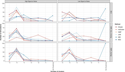
Ability to recover the correct number of simulated clusters: number of shared clusters estimated in each simulation scenario (rows) and SNR (columns).
The number of clusters estimated by each method on the 600 simulations is shown in Figure 1. We recall that each simulation consists of three data sets sharing three global clusters, as described in Simulation scenarios. One can first notice that the methods correctly retrieved three clusters on average. The distributions appear sharper around the modes for the high SNR and the iNMF-overlap scenario. Conversely, the methods globally perform poorly on the iNMF-non-overlap scenario, probably because these simulations contain the same number of shared and specific variables, and that common blocks have half as many variables as those in the iNMF-overlap scenario. Continuing with the iNMF-non-overlap scenario, the estimated number of clusters is uniform for moCluster and JIVE, while it successfully peaks around three clusters for iCluster and BCC. These observations suggest that the latter are more robust to the reduction of shared blocks. On BCC simulations, unlike matrix factorization approaches, the two Bayesian methods either do not detect clusters (MDI) or fail to identify the three global clusters (BCC). These results are surprising since one would expect a method run on simulations generated with its own model to perform well. The systematic absence of clustering returned by MDI for low SNR simulations, regardless of the scenario, implies that the method lacks robustness against noise. One can finally note systematic biases in four methods: iNMF and iCluster on the one hand, moCluster and MDI on the other hand suffer from under and over-estimation, respectively. This is particularly true on BCC and iNMF-non-overlap simulations. Overall, iNMF, iCluster, JIVE, BCC, moCluster and MDI successfully recovered three clusters in 62.7, 55.7, 55.5, 44.5, 43.5 and 21.8% of the simulations respectively.
Method performances on shared and specific structures
After evaluating the methods’ ability to estimate the number of clusters, we now assess the clustering quality by measuring the coherence between simulated and estimated clusterings both at the shared and data-specific levels. In this analysis, methods were configured so that the expected number of clusters are set to the true number of simulated clusters, except for Bayesian approaches on specific clusters. Indeed, the specific clustering depends on the simulation, matrix and method considered. The dependence on the method exists because specific structures are modeled differently in matrix factorization and Bayesian methods. This modeling difference only arises in iNMF simulations when a specific block overlap with two common blocks; in this situation, matrix factorization methods (JIVE and iNMF) are designed to recover all three blocks (two common and one specific clusters), whereas Bayesian approaches see three specific clusters. Therefore, when computing ARI for specific structures, the expected clustering was provided by unique blocks in |$\textit {Z}^s_k$| or |$\textit {Z} + \textit {Z}^s_k$| when run with matrix factorization or Bayesian approaches, respectively. Similarly, the number of specific clusters was set to the number of these unique blocks.
To guarantee a fair comparison across methods, the parameters were set to their best-performing values defined as either the value used in data simulation or the ones maximizing the ARI with the global clustering. Indeed, some parameters were straightforward to set because fixed in the simulations, namely, the number of common and specific clusters as well as the number of latent variables in iCluster and moCluster [|$\text {rank}(\textit {Z}) = 2$|]. For the others, i.e. the number of latent variables in JIVE, the number of modules and the homogeneity level in iNMF, the maximum number of clusters |$q$| in BCC, a grid search aiming at finding the parameters maximizing the ARI was conducted. Certain parameters in iNMF (homogeneity) and BCC (maximum number of clusters) could favor the common or specific structure over the other. Since the goal in data integration is to identify common variations, the parameters were tuned to maximize the ARI of the global clustering.
Supplementary Figures 2–4 display the performances of these three methods on the common and specific structures for all simulation scenarios. Starting with JIVE, the rank does not show much effect on the method performances. For the specific structures, ARIs are under 0.25, indicating a poor ability to recover them. For the shared structures, ARIs appear on average slightly higher when rank equals 2, value retained in the method comparison. For iNMF, a clear increase in ARI between two and three modules followed by a plateau led to the selection of three modules. Unsurprisingly, the homogeneity parameter has a large impact on the recovery of the shared or specific structures, trend particularly apparent on BCC simulations where the largest (resp. smallest) homogeneity value allows an almost perfect identification of the common (resp. specific) structures (ARI |$\approx$|1). The selected homogeneity value was the one favoring most the common structure, i.e. |$\lambda = 0.3$|. Similarly, Supplementary Figure 4 reveals an important effect of the number of clusters on BCC performances for the first two simulation scenarios: a bell-shaped curve peaking at three clusters is obtained with iNMF simulations, while the highest ARIs are attained when the number of clusters was set to this used in simulations (‘As Simulated’) for BCC simulations and this for both shared and specific structures. By contrast, the ARI shows almost no variations across cluster numbers on the sensitivity scenario. Those parameter values selected by grid search or from the simulation design are summarized in Table 2.
Best-performing parameters selected by grid search before method comparison. The ranges tested for each parameter are indicated in parenthesis (see Supplementary Figures 2–4)
| JIVE | iNMF | BCC | ||
|---|---|---|---|---|
| Number of latent variables / modules | 2 (2–5) | 3 (2–6) | – | |
| Homogeneity level | – | 0.3 (0.01,0.03,0.1,0.3) | – | |
| Number of clusters | iNMF simulations | – | – | 3 (2–7 and ‘as simulated’) |
| BCC simulations | – | – | as simulated (2–7 and ‘as simulated’) |
We now turn to the method comparison at the shared level. In addition to the six integrative methods, two alternatives mentioned in the introduction were included to evaluate the added value of integration: consensus clustering based on maximization of the PEAR [38] and Gaussian mixture model (GMM) clustering on concatenated matrices using the Mclust R package. It can first be noticed that most integrative methods display high ARI, suggesting a good ability to recover common clusters (Figure 2a). The SNR has a large impact on the performances, especially on MDI and the concatenation approach (BCC simulations only), which both lack robustness against noise. Similar trends are observed in overlap and non-overlap-iNMF simulations where matrix factorization approaches have equivalent ARI and outperform Bayesian methods, while non-integrative approaches show smaller ARI. Similarly to the previous section, the performances decrease in iNMF-non-overlap simulations, which can again be attributed to the fact that common blocks contain half as many variables as in the overlap scenario. This drop is more accentuated with MDI, supporting the idea that the method is more sensitive to data perturbations. Looking at BCC simulations, iCluster, moCluster and iNMF outperform again the others, shortly followed by consensus clustering, JIVE and BCC. Matrix concatenation and MDI, on the other hand, show relatively large ARIs when SNR is high but perform poorly at low SNR.
The results with matrix concatenation are in line with the previous study [9]. Overall, matrix factorization methods and, more particularly, iCluster, moCluster and iNMF present the best ability to recover common structures, and, this, regardless of the simulation scenario. BCC shows an intermediate behavior between matrix factorization approaches and MDI. Despite a moderate robustness when shared and specific blocks do not overlap, BCC displays fairly high ARIs on BCC simulations, probably because the simulations were generated from the same model.
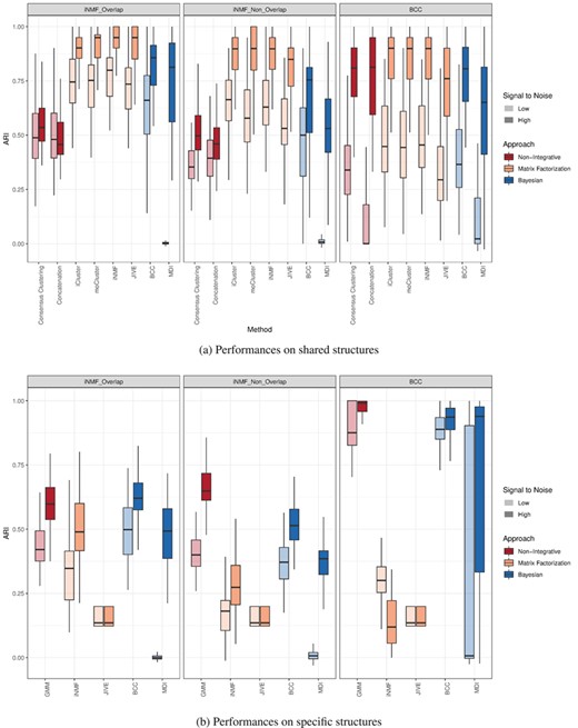
Consistency between simulated and estimated clusterings: ARI boxplots are displayed on shared (a) and specific (b) structures for each simulation scenario (columns) and SNR (transparency).
The detection of data-specific structures is not central in this study given that standard clustering approaches are tailored for this task. We nevertheless evaluated this functionality because one is generally interested in both shared and specific structures when performing multi-omic studies. Similarly to the evaluation of the shared structures, GMM was added in the comparison to benchmark the four methods against a standard (non-integrative) clustering approach. In the two simulation scenarios, GMM, closely followed by BCC, outperforms the 3 other integrative methods with ARIs close to one in BCC simulations (Figure 2b). Matrix factorization methods, JIVE in particular, performs poorly in all scenarios. In the same way as the shared structure evaluation, MDI achieves close to zero ARI at low SNR confirming its lack of robustness to noise but nevertheless showed intermediate ARI values at high SNR. These results are not unexpected since GMM and BCC are designed focus on data-specific clustering, whereas iNMF and JIVE aim to recover shared clusters.
To conclude on this section, the six methods showed a real improvement over non-integrative approaches to find shared clusters on iNMF simulations, while only iCluster, moCluster and iNMF did so on BCC simulations. By contrast, the methods failed to reach GMM performances on specific clusters, except for BCC. Unsurprisingly, no method could properly identify shared and specific structures simultaneously. Because the detection of either structure is largely influenced by parameters, the latter must be carefully tuned according to the study goals. The same trends were also observed in the iNMF-high-dimensional scenario, which indicates that the results also apply in high dimension, when the number of features differs across data sets (Supplementary Figures 5–7).
Evaluation of methods sensitivity
The present study of sensitivity aims at determining whether the methods accurately identify common structures when their size is reduced up to |$n_b=5$| samples per block. No additional tuning step was required as parameters were determined for all scenarios, including the sensitivity ones, in the previous section. Only the number of expected clusters was changed to 4 when |$n_b\leq 17$|, i.e. when a noise cluster was present.
As already noticed in the previous results, SNR and overlaps across structures largely influence the performances, especially at |$n_b=5$| where ARIs are roughly twice as large in the iNMF-overlap as in the iNMF-non-overlap scenario (Figure 3). As expected, the size of the blocks also impacts the performances, with ARIs increasing with the number of samples per block. Surprisingly, this trend is not linear at high SNR where performances successively increase (|$n_b\in \{5,8\}$|), plateau or slightly drop (|$n_b\in \{8,17\}$|) and increase again (|$n_b\in \{17,20\}$|). To rule out possible simulation errors, the median ratio of between to total sum of squares (BSS/TSS) was computed for each block size. The resulting BSS/TSS correlated almost perfectly with the blocks sizes (|$r=0.94, 0.99$| for overlapping and non-overlapping scenarios, respectively), excluding thus this hypothesis. A literature review on clustering evaluation indices revealed that most of the existing measures, ARI included, are sensitive to class size unbalance [39]. Given that the noise cluster makes up from 0–75% of the simulations, we can suspect that such unbalance between signal and noise clusters is responsible for the observed behavior. The fact that this trend does not occur at low SNR, however, questions this explanation or suggests that the unbalance effect has a smaller impact at low SNR.
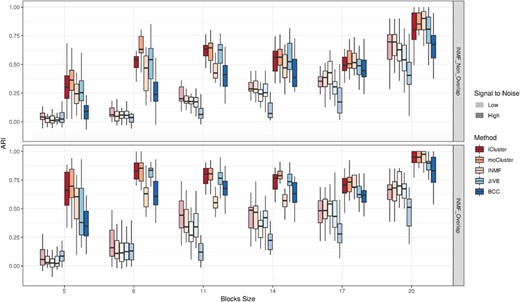
Evaluation of methods’ sensitivity: ARI distributions are displayed for different block sizes (|$n_b \in \{5,8,11,14,17,20\}$|), simulation scenarios (rows) and SNRs (transparency).
The hierarchy among methods is similar between blocks sizes, SNR levels and structures. iCluster and moCluster show the highest ARIs when |$n_b<20$| and remain high at |$n_b=20$|. JIVE displays a sensitivity close to these two methods for all blocks sizes. iNMF and BCC, on the other hand, are the least sensitive with, however, a sharp improvement of iNMF for |$n_b=20$|. Lastly, MDI did not return any results for |$n_b<20$|, which again supports its lack of robustness against perturbations. Although the results with |$n_b=20$| are consistent with those obtained in Methods overview, they are not exactly equal since the numbers of variables (see Supplementary Materials) and repetitions by block size are slightly different.
Application: TCGA breast cancer data set
We now examine how the six methods compare on the TCGA breast cancer data set [2], the TCGA data being extensively used in the evaluation of integrative approaches [24, 26, 28, 30, 35]. The breast cancer data set consists of SNP, RNA, miRNA, DNA methylation and protein (reverse phase protein array) measurements in 825 patients. Here, the analysis is based on a subset of 348 patients assayed across all platforms, for which data were imputed and pre-processed by the authors of BCC (see BayesCC R package). Of note, SNP data were left aside by the authors. Because cancers are heterogeneous diseases, the diagnostic accuracy is essential for both the prognostic and the choice of treatment. The American Cancer Society classifies breast cancer into four molecular subtypes, HER2 enriched, basal (triple negative) and luminal A and B, based on the expression of proliferating protein Ki67 and the receptor status for estrogen (ER), progesterone (PR) and human epidermal growth factor 2 (HER2), as described in Table 3. Because tumors with similar immunohistochemistry and clinicopathological profiles may have different behaviors, recent omic approaches have sought to refine this classification by identifying new molecular signatures [40]. However, given that no consensus has emerged yet, we will consider the classification from the American Cancer Society (used in clinics) as gold standard and evaluate the integrative methods based on their consistency with subtypes derived from the receptor status.
Breast cancer subtypes as defined by the American Cancer Society [41]
| Subtype | Markers status |
|---|---|
| ER− | |
| Basal | PR− |
| HER2− | |
| ER− | |
| HER2 | PR− |
| HER2|$+$| | |
| ER|$+$| and/or PR|$+$| | |
| Luminal A | HER2− |
| ER|$+$| and/or PR|$+$| | |
| Luminal B | HER2|$+$| or High Ki67 |
| Subtype | Markers status |
|---|---|
| ER− | |
| Basal | PR− |
| HER2− | |
| ER− | |
| HER2 | PR− |
| HER2|$+$| | |
| ER|$+$| and/or PR|$+$| | |
| Luminal A | HER2− |
| ER|$+$| and/or PR|$+$| | |
| Luminal B | HER2|$+$| or High Ki67 |
Since Ki67 was missing in the data, luminal A and B subtypes could not be distinguished. For this reason, although integrative methods were run with 4 clusters on 348 patients, only the 84 patients annotated as basal and HER2 from the clinical data were kept in the computation of ARI. Similarly to the simulation studies, consensus clustering, GMM clustering on concatenated matrices and GMM clustering on single omics were included in the comparison.
On Table 4, one can note that single-omic clusterings display a wide range of performances, suggesting that these omics are not impacted similarly during carcinogenesis. However, it cannot be excluded that this result is due to the higher number of features measured in mRNA and DNA methylation. Unexpectedly, a null ARI was found with proteins, which can be attributed to the high cluster unbalance obtained with GMM in this omic. Although these observations contrast with the high concordance between protein and mRNA subtypes reported in the original study [2], this may arise from a difference of samples used, our analysis being based on patients assayed on all platforms.
Cluster profiles in terms of receptor percentages; consistency (ARI) between cancer subtypes and estimated clusterings. Clusters are colored according to their similarity to the 4 subtypes defined Table 3
| Method | %ER | %PR | %HER2 | ARI |
|---|---|---|---|---|
| Consensus clustering | 97 | 89 | 11 | 0.52 |
| 66 | 45 | 38 | ||
| 11 | 5 | 2 | ||
| 96 | 80 | 16 | ||
| Concatenation | 97 | 89 | 7 | 0.52 |
| 98 | 77 | 22 | ||
| 13 | 6 | 2 | ||
| 63 | 44 | 41 | ||
| iCluster | 95 | 71 | 26 | 0.42 |
| 96 | 85 | 8 | ||
| 90 | 81 | 18 | ||
| 12 | 5 | 9 | ||
| moCluster | 13 | 6 | 2 | 0.57 |
| 98 | 83 | 8 | ||
| 64 | 40 | 56 | ||
| 96 | 89 | 9 | ||
| iNMF | 8 | 56 | 41 | 0.56 |
| 97 | 9 | 6 | ||
| 13 | 6 | 7 | ||
| 100 | 87 | 8 | ||
| JIVE | 96 | 84 | 9 | 0.40 |
| 12 | 4 | 7 | ||
| 99 | 84 | 6 | ||
| 79 | 63 | 39 | ||
| BCC | 70 | 49 | 43 | 0.51 |
| 18 | 9 | 4 | ||
| 97 | 84 | 10 | ||
| 98 | 89 | 9 | ||
| MDI | 94 | 87 | 10 | 0.55 |
| 14 | 8 | 3 | ||
| 100 | 94 | 19 | ||
| 99 | 83 | 10 | ||
| mRNAs | – | 0.50 | ||
| DNA methylations | – | 0.41 | ||
| miRNAs | – | 0.30 | ||
| Proteins | – | 0.00 | ||
In line with the simulation results, all integrative methods but iCluster and JIVE outperformed single-omic approaches. The hierarchy among methods slightly differs with this obtained in the simulations; although moCluster and iNMF remain the top performing methods, they are closely followed by MDI then non-integrative approaches and BCC. iCluster and JIVE, on the other hand, present ARI 0.1 to 0.17 smaller than the others.
We then manually assigned (colored) clusters to their most plausible subtype based on Table 3: clusters with small percentages for all receptors were classified as basal, whereas those with high percentages of ER and PR were assigned to luminal A/B. As indicated above, luminal A and B clusters were merged due to the absence of Ki67 in the data. All methods successfully identified one basal and one to three luminal clusters, but none recovered the HER2 subtype. The absence of HER2 cluster and the over-representation of luminal ones are probably due to their subtype prevalence, larger in the former [41]. Six methods identified another cluster with average percentage values for all receptors; although matching no subtype, this cluster is most likely a mixture of HER2 and luminal patients. Because the eight approaches identified the four expected subtypes with a comparable, moderate accuracy, this step did not allow to further refine the method hierarchy.
In the same way as the simulations, this application confirmed that integrative approaches have an improved ability to identify common structures over single omics. Although moCluster and iNMF came first, Bayesian approaches surpassed iCluster and JIVE, in contrast with the results obtained in the simulations. We can, however, suppose that the use of sparsity could significantly improve the results of the latter.
Discussion and conclusion
Six popular integrative clustering methods, representative of matrix factorization and Bayesian approaches, were compared on simulations based on their (i) sensitivity and their ability to recover the (ii) number of clusters, (iii) common and specific structures across three data sets. Different simulation scenarios based on 12 combinations of models, SNR, data set dimension (iNMF-high-dimensional, sensitivity study) and overlaps between common and specific structures were tested to unveil methods’ strengths and limitations.
The results from the simulations and application revealed that matrix factorization methods were on average better at identifying both common structures and the correct number of clusters; iCluster and moCluster outperformed the other methods on all criteria except on the application (iCluster) or the enumeration of the number of clusters (moCluster). Despite a probable lack of sensitivity, iNMF also showed a great ability to detect common clusterings and offered a homogeneity parameter, allowing the user to finely tune the matrix factorization between shared and specific structures, as depicted in Supplementary Figure 3. JIVE was generally close to the other matrix factorization methods, with however lower performances on the application and the detection of specific clusters. While BCC revealed a good ability to identify common structures, except on the iNMF-non-overlap and sensitivity scenarios, its main strength resides in its capability to simultaneously detect shared and specific structures. Lastly, MDI showed good performances in high SNR simulations and the application but had little robustness against data perturbations (noise and overlap between shared and specific structures). Of note, despite their longer runtime, the two Bayesian approaches were easier to parametrize. Additionally, we showed that neither the dimensionality nor the unbalanced number of features across data sets had an impact on the results. Some limitations of our work must be acknowledged. First, the evaluation criterion utilized throughout this work was the coherence between known and estimated sample clustering. A similar evaluation could also be performed at the variable level. Second, because a fair amount of time was invested in parameter tuning, we decided not to include feature selection in it. It would however be worth investigating the effect of penalization on the method performances. Third, although we highlighted pros and cons of these six methods through various simulation scenarios, method robustness could also have been evaluated by adding noise variables in varying proportions.
In addition to the presented benchmarking, our work demonstrated on all simulations the advantage of integrative methods over non-integrative ones in the identification of common structure, supporting their use in the identification of complex structures across omic layers.
The integration of multiple omics shows a clear improvement in clustering performance as compared to non-integrative methods.
Matrix factorization methods are on average better at identifying common structure.
Although iNMF showed a lack of sensitivity, it can finely be tuned to recover either common or specific structures.
Despite moderate performances on shared clusters, BCC displayed the best ability to recover both structures simultaneously.
Acknowledgments
We thank Vivian Viallon for helpful discussions. We also thank the IN2P3 Computing Center (Centre National de la Recherche Scientifique, Lyon-Villeurbanne, France) for providing high performing infrastructure.
Funding
BIOASTER investment funding (ANR-10-AIRT-03).
Cécile Chauvel, PhD, is a researcher in biostatistics in the Data Management and Analysis unit at Bioaster, Lyon, France.
Alexei Novoloaca is a PhD student in biostatistics in the Epigenetics Group at the International Agency for Research on Cancer, World Health Organization, Lyon, France.
Pierre Veyre is a computer scientist in the Data Management and Analysis unit at Bioaster, Lyon, France.
Frédéric Reynier, PhD, is the head of the Genomics and Transcriptomics unit at Bioaster, Lyon, France.
Jérémie Becker, DPhil, is a researcher in biostatistics in the Genomics and Transcriptomics unit at Bioaster, Lyon, France. BIOASTER is a technological research institute in microbiology that aims to develop new innovative and high-value technology solutions through collaborative projects. Its main interest lies in tackling antimicrobial resistance, developing new diagnostics, improving vaccines’ safety and efficacy and understanding the involvement of microbiome in human and animal health.
References
Author notes
The authors wish it to be known that, in their opinion, the first two authors should be regarded as joint First Authors.
