


Abstract
We present here an integrated analysis of structures and functions of genome-scale metabolic networks of 17 microorganisms. Our structural analyses of these networks revealed that the node degree of each network, represented as a (simplified) reaction network, follows a power-law distribution, and the clustering coefficient of each network has a positive correlation with the corresponding node degree. Together, these properties imply that each network has exactly one large and densely connected subnetwork or core. Further analyses revealed that each network consists of three functionally distinct subnetworks: (i) a core, consisting of a large number of directed reaction cycles of enzymes for interconversions among intermediate metabolites; (ii) a catabolic module, with a largely layered structure consisting of mostly catabolic enzymes; (iii) an anabolic module with a similar structure consisting of virtually all anabolic genes; and (iv) the three subnetworks cover on average ∼56, ∼31 and ∼13% of a network’s nodes across the 17 networks, respectively. Functional analyses suggest: (1) cellular metabolic fluxes generally go from the catabolic module to the core for substantial interconversions, then the flux directions to anabolic module appear to be determined by input nutrient levels as well as a set of precursors needed for macromolecule syntheses; and (2) enzymes in each subnetwork have characteristic ranges of kinetic parameters, suggesting optimized metabolic and regulatory relationships among the three subnetworks.
Introduction
Metabolism refers to operation of chemical reaction chains essential to sustaining life of a living organism, specifically for converting nutrients to energy and biomolecules needed for cellular housekeeping, stress response, proliferation and waste processing [1, 2]. Each metabolic reaction is typically catalyzed by one or several enzymes. Under different conditions, distinct components of a metabolic system may be activated in response to the perceived changes in intracellular or extracellular environment [3, 4]. Currently, our understanding of the entire metabolic system of a cell, even for the simplest bacterial cell, remains largely at the level of individual metabolic pathways and coordinated activities among different pathways. We are yet to understand how these pathways are functionally connected to work as a system in a condition-dependent manner, e.g. how different components of a metabolic system complement and compensate for each other under varying nutrient or stress conditions.
Because of high intrinsic complexities of metabolic networks, genome-scale metabolic studies are generally conducted through mathematical or computational analyses, by first representing a complex reaction system as a metabolic network [5, 6], followed by topological analyses of such a network [7–10] and/or flux analyses of the network via elementary flux mode analysis [11, 12] coupled with flux balance analyses (FBAs) [13, 14] or more sophisticated analyses that use kinetic and/or thermodynamic information as flux constraints [15, 16]. Three approaches have been widely used to represent a metabolic network: (a) metabolite networks that represent the metabolites as nodes and reactions as edges [7, 8, 10]; (b) reaction networks with reactions represented as nodes and metabolites as edges [8, 9, 17]; and (c) bipartite networks, where both metabolites and reactions are modeled as nodes and an edge connects a reaction with a metabolite if the reaction involves the metabolite [18].
Various properties of the represented networks have been studied. Two parameters, namely, node degree and clustering coefficient [19, 20], have been often used to analyze the topological properties of such networks, just like other networks such as social networks, Internet and electric power grids. Previous studies have demonstrated that metabolite networks generally have a hierarchical architecture; and their node degree and clustering coefficient follow power-law distributions [7]. It was noteworthy that some properties may not be easily observable when a metabolic system is represented in other formats [21, 22]. A challenging issue is: What information should be represented in a metabolic network, which is essential to elucidating the fundamental properties of metabolic systems, such as the principles of their organization and operation? For example, it has been noted that it may considerably alter the ‘basic’ properties of a network when currency metabolites such as ATP or NAD/NADH, which are widely used in enzymatic reactions, are treated as regular metabolites in a reaction network. Such altered properties include, for example, whether the node degrees and clustering coefficient of a network follows a power-law distribution [22–24], whether a metabolic network forms one, two or more large and densely connected subnetworks [9, 25, 26]. It is noteworthy that such topological studies of metabolic networks start to offer useful information to functional studies of microbial metabolism. For example, metabolic fluxes derived using traditional FBAs tend to suffer from low-accuracy issues, and the prediction accuracy can be improved when constrained with growth condition-specific network topology information [27, 28]. Specifically, it has been demonstrated that an improved network topology design can improve the yield of desired bio-product [29, 30].
In this article, we present a computational analysis of microbial metabolic networks, aiming to better understand the organizing and operating principles of microbial metabolism. Specifically, we address the following issues: (i) representation of a metabolic network as a simplified reaction network (SRN) to reveal the fundamental structures of a metabolic network to enable reliable flux analyses; (ii) derivation of key topological properties of the reaction networks; and (iii) inference of how such topological properties, coupled with empirical kinetic parameters of enzymes in distinct subnetworks for optimal functions of microbial metabolism. We anticipate that the insights gained here will inform studies of microbial metabolism.
Results
Genome-scale metabolic networks of 17 microbial organisms: 15 bacterial, 1 archaeal and 1 single-cell eukaryotic organisms, are selected and analyzed here (see ‘Materials and methods’ section) to derive key topological properties and apply the properties to functional analyses.
Elucidation of the organizing principles of microbial metabolic networks
Network properties without considering currency metabolites
In any metabolic system, some enzymes require currency metabolites such as ATP, NADPH or Fe2+, to be activated from their inactive states. These currency metabolites are each involved in large fractions of all the enzymatic reactions, hence making significant contributions to the structure and the complexity of a reaction network. Previous studies have suggested that inclusion of currency metabolites in network topology analyses may not be justified because of their ubiquitous nature in contributing to enzymatic reactions [31]. Based on this consideration, we have removed 28 currency metabolites (see ‘Materials and methods’ section, and Supplementary Figure S1A) from our network representation. We refer to the resulting networks as currency metabolites-free networks.
We found the node degree in each of the 17 currency metabolites-free networks follows a power-law distribution with an average exponent1.623 (Figure 1A–E and Supplementary Figure S2), which is lower than for a typical scale-free network [19, 32] and higher than the average value 1.42 of less complete networks [8, 9, 17], with being a positive constant. In addition, the average clustering coefficient across the 17 networks is (paired t-test, P < 1.14E-19), compared with 0.348 of the original metabolic networks (without the removal of currency metabolites, which are not scale-free) (Figure 1F); and the average shortest path length within each network is 7.18 (paired t-test, P < 1.26E-19), compared with 2.63 of the original networks (Supplementary Tables S1 and S2). It is noteworthy that the effect of removing currency metabolites on network topology has been assessed previously [17], but their results may not be accurate, as the networks used in the analyses tend to be substantially less complete compared with the ones used here.
![Node degree and clustering coefficient statistics. (A–D) Power-law distribution of the currency metabolites-free reaction network (CFF) (red line) and the SRN (blue line) of E. coli K-12, Klebsiella pneumoniae, Salmonella enterica serovar and Yersinia pestis, respectively. In each panel, the x-axis represents the log-transformed values of node degrees, and the y-axis denotes the frequencies of each x-value. (E) Comparison between the exponent values in the power-law distributions of node degrees in CFF versus SRN networks of the 17 species (n = 32; two-tailed Student’s t-test, P < 4.37E-5). (F) Comparison among clustering coefficients of the original reaction networks, CFFs and SRNs of the 17 species (n = 32; two-tailed Student’s t-test, *P <1.14E-19, **P < 9.31E-6). (G) The clustering coefficient distribution of the E. coli K12 network is considerably different from those of the BA scale-free networks (n = 3605; two-tailed Student’s t-test, *P <2.38E-7) [19], which have the same node degree distribution with those of the SRN networks.](https://oup.silverchair-cdn.com/oup/backfile/Content_public/Journal/bib/20/4/10.1093_bib_bby022/2/m_bby022f1.jpeg?Expires=1749146733&Signature=fkoOKhb7D4MgYVE8UzQJsVuqg34LfFYPRGUqAUlc6ADBfT1kzk-ze2VtDEd7tAuQjQoN7AVmhbFzCaSC9fIG7CS3h8SOrhSaV6j~Mk~AzrSpANI2NQmWv3bbsmdfTgn5ikvavhAYgVSdWc46Iy0bsT47D6s2rXiXPqVNIsHN~g-pLH3Tf8lG9RmsokBq9x4THjdrzueOcgmMlbb7gxhF7Nyam2ii3zNXaAV~YGIaffLeMAihs06JfyzQW8MT3Qm2nFG7pOvQOvNMQVNnAuhBuab9Uq5qjmHXfaA8DhmNk59yWH5hZhoP0URdSKFBfHKmjBReEBN~xA0nFdjEzgsXaQ__&Key-Pair-Id=APKAIE5G5CRDK6RD3PGA)
Node degree and clustering coefficient statistics. (A–D) Power-law distribution of the currency metabolites-free reaction network (CFF) (red line) and the SRN (blue line) of E. coli K-12, Klebsiella pneumoniae, Salmonella enterica serovar and Yersinia pestis, respectively. In each panel, the x-axis represents the log-transformed values of node degrees, and the y-axis denotes the frequencies of each x-value. (E) Comparison between the exponent values in the power-law distributions of node degrees in CFF versus SRN networks of the 17 species (n = 32; two-tailed Student’s t-test, P < 4.37E-5). (F) Comparison among clustering coefficients of the original reaction networks, CFFs and SRNs of the 17 species (n = 32; two-tailed Student’s t-test, *P <1.14E-19, **P < 9.31E-6). (G) The clustering coefficient distribution of the E. coli K12 network is considerably different from those of the BA scale-free networks (n = 3605; two-tailed Student’s t-test, *P <2.38E-7) [19], which have the same node degree distribution with those of the SRN networks.
While the currency metabolite removal has given rise to reaction networks with node degrees following power-law distributions, similar to those of well-studied scale-free networks such as the World Wide Web or protein–protein interaction networks [19, 32]; the exponent values of scale-free networks are considerably lower than the values in the reaction networks. This, coupled with the observation that the clustering coefficient of each currency metabolites-free network under consideration does not follow a power-law distribution and is larger than those of Barabási–Albert (BA) scale-free networks (Figure 1G), indicates that reaction networks have more densely connected hub nodes than the previously studied scale-free networks. Our further analysis revealed that the 17 networks each consists of two large densely connected subnetworks as shown in Figure 2 and Supplementary Figure S3, and the similar results were also observed according Chen et al. [25]. Our question is: What gives rise to this characteristic of these currency metabolites-free networks?
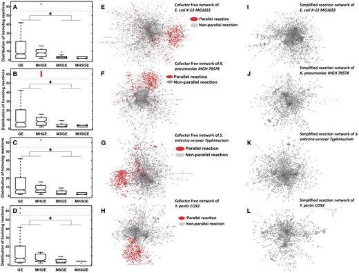
Simplified reaction networks. (A–D) The number of reactions catalyzed by specific types of enzymes in E. coli K-12 (n = 1258, two-tailed Student’s t-test, *P <1.27E-11), K. pneumoniae MGH (n = 1227, two-tailed Student’s t-test,*P <6.92E-5), S. enterica serovar (n = 1269, two-tailed Student’s t-test, *P <4.74E-11) and Y. pestis (n = 813, two-tailed Student’s t-test, *P <1.19E-6), respectively, where GE is for the set of reactions each catalyzed by exactly one enzyme; MHGE is for reactions each catalyzed by anyone in a group of homologous enzymes; MSGE for reactions each catalyzed by multiple enzymes; and MHSGE for reactions each catalyzed by any set of multiple enzymes in a collection of multiple such sets. (E–H) Highlighted parallel reactions in the currency metabolites-free reaction network for each of the four species. (I–L) SRN containing one large and dense subnetwork for each of the four species.
Further simplification of networks by collapsing parallel reactions into one
Nam et al. [33] classified enzymes into generalists and specialists based on the number of reactions that an enzyme catalyzes. Our analyses revealed that monomeric enzymes encoded in a genome tend to catalyze more (distinct) reactions, specifically 10.81 reactions per monomeric enzyme compared to 4.25 reactions per multimeric enzyme, which has two or more component proteins on average (paired t-test, P < 1.12E-7) (Figure 2A–D and Supplementary Figure S4 and Supplementary Table S4). This observation suggests that reactions sharing similar substrates and products have high probabilities being catalyzed by monomeric enzymes than multimeric ones (Supplementary Data S1). Such reactions are referred to as parallel reactions. Interestingly, one of the two large, densely connected subnetworks mentioned above predominantly consists of such parallel reactions (Figure 2E–H and Supplementary Figure S3). By identifying all sets of parallel reactions and collapsing each into one reaction (see ‘Materials and methods’ section), the complexity of each of the 17 reaction networks is substantially reduced, and the second largest densely connected subnetwork disappears in all networks.
We have further observed that redundant edges will be introduced when representing two consecutive reversible reactions with one using the products of the other one as the substrates in a reaction network. By identifying and removing such redundant edges (see ‘Materials and methods’ section), we have further reduced the complexity of the reaction networks. Specifically, each reaction network now consists of only one large, densely connected subnetwork (Figure 2I–L), named a SRN. The average exponent γ value of the node degree distribution increases to 1.88 from 1.62 (paired t-test; P < 4.37E-5) for the currency metabolites-free networks, and the average clustering coefficient decreases to 0.109 from 0.166 (paired t-test; P < 9.31E-6), along with the average shortest path having 7.33 nodes, increased from 7.18 as given in Figure 1A–F (and Supplementary Tables S2 and S4).
Network incompleteness and implications
It is noteworthy that the 17 metabolic networks studied here are incomplete because of the limitation in current knowledge of microbial metabolism. We have estimated the level of incompleteness of each of the 17 networks and demonstrated how the level of incompleteness may have affected the estimated parameters above. Specifically, two ratios are used to estimate the level of a network’s incompleteness: the ratio between the number of metabolites and the number of reactions, represented as, and the ratio between the number of identified metabolic genes and the total number of genes encoded in each genome, denoted as . Note that the lower the value, the more complete a network is, and similarly, the higher thevalue, the more complete a network is (see ‘Materials and methods’ section). Figure 3 shows the detailed relationship between each ratio and the clustering coefficient as well as the exponent γ value in the corresponding power-law distribution of the node degrees.
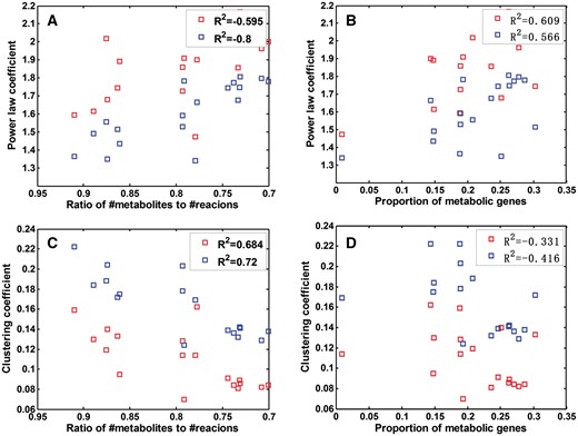
The exponent in the node degree distribution and clustering coefficient versus network completeness. In each penal, a blue square is for a currency metabolites-free network of the 17 species, and each red square is for an SRN, respectively. The value R2 is the squared Pearson correlation coefficient. (A) The value versus . (B) The value versus . (C) The clustering coefficient versus . (D) The clustering coefficient versus Note the x-axis of panels of A and C are ordered from high to low values.
A lasso regression was conducted on γ against the estimated levels of incompleteness using the two ratios, across the 17 networks, to derive a quantitative estimate of how the level of a network’s incompleteness affects the above estimated parameters of a network. A similar analysis was carried on clustering coefficients against the estimated levels of network incompleteness. The two models have R2 = 0.695 (F test, P < 1.0E-4) and R2 = 0.628 (F test, P < 6.0E-4), respectively, where R2 is the squared Pearson correlation coefficient. Based on the derived relationships between γ and the estimated level of incompleteness as well as between the clustering coefficient and the level of incompleteness, we have reestimated the two topological parameters for the 17 reaction networks through extrapolating the models to the corresponding complete networks; and obtained an average γ value 2.006 and an average clustering coefficient 0.085 across the 17 networks if they were complete (Table 1). Figure 3 shows that the observed correlation between the level of a network’s completeness and the estimated topological parameters is because of the intrinsic properties of the metabolic networks instead of the simplification in our representations of the networks.
Statistics about network completeness and our regression results for the 17 reaction networks, where are the exponent of the power-law distribution and the average clustering coefficient of a reaction network, respectively
| Organism | Parameters | Result | |||||||
|---|---|---|---|---|---|---|---|---|---|
| #Metabolites | #Reactions | #Metabolic genes | #All genes | #Predicted metabolic reactions | |||||
| Bacillus subtilis 168 | 991 | 1250 | 0.792 | 844 | 4454 | 0.189 | 2400 | 2.019 | 0.084 |
| Clostridium ljungdahlii DSM 13528 | 698 | 785 | 0.889 | 637 | 4283 | 0.148 | 2400 | 2.013 | 0.084 |
| Escherichia coli K-12 MG1655 | 1668 | 2382 | 0.7 | 1260 | 4400 | 0.286 | 2400 | 2.0063 | 0.084 |
| Geobacter metallireducens GS-15 | 1109 | 1285 | 0.863 | 987 | 3260 | 0.302 | 2150 | 1.92 | 0.087 |
| Helicobacter pylori 26695 | 485 | 554 | 0.875 | 339 | 1632 | 0.207 | 1000 | 1.88 | 0.103 |
| Klebsiella pneumoniae MGH 78578 | 1658 | 2262 | 0.732 | 1229 | 5211 | 0.235 | 2900 | 2.19 | 0.077 |
| Methanosarcina barkeri str. Fusaro | 628 | 690 | 0.91 | 692 | 3679 | 0.188 | 2200 | 1.94 | 0.087 |
| Pseudomonas putida KT2440 | 909 | 1056 | 0.86 | 746 | 5046 | 0.147 | 2700 | 2.12 | 0.08 |
| Saccharomyces cerevisiae S288c | 1226 | 1577 | 0.777 | 905 | 6275 | 0.009 | 3000 | 2.22 | 0.075 |
| Salmonella enterica serovar Typhimurium | 1802 | 2545 | 0.708 | 1271 | 4569 | 0.278 | 2500 | 2.049 | 0.082 |
| Shigella boydii CDC 3083-94 | 1912 | 2592 | 0.737 | 1147 | 4244 | 0.27 | 2300 | 1.97 | 0.085 |
| Shigella dysenteriae Sd197 | 1890 | 2540 | 0.744 | 1059 | 4294 | 0.246 | 2300 | 2.001 | 0.085 |
| Shigella flexneri 2a 2457T | 1914 | 2620 | 0.73 | 1180 | 4491 | 0.262 | 2440 | 2.027 | 0.083 |
| Shigella flexneri 5 8401 | 1917 | 2622 | 0.731 | 1184 | 4491 | 0.263 | 2400 | 2.02 | 0.084 |
| Staphylococcus aureus N315 | 665 | 743 | 0.89 | 619 | 2872 | 0.215 | 1600 | 1.89 | 0.084 |
| Thermotoga maritima MSB8 | 570 | 652 | 0.874 | 482 | 1921 | 0.25 | 1040 | 1.82 | 0.1 |
| Yersinia pestis CO92 | 1552 | 1961 | 0.791 | 815 | 4218 | 0.193 | 2400 | 2.012 | 0.084 |
Understanding the structural organization of metabolic networks based on clustering coefficients
Previous studies have found that the clustering coefficients of metabolite networks follow power-law distributions [7]. In comparison, all the 17 reaction networks each display a positive correlation between the clustering coefficient and the node degree (Figure 4A–D and Supplementary Figure S5), which is distinct from both the metabolite networks and the widely studied BA scale-free networks, whose clustering coefficients are independent of node degrees, as shown in Figures 1G and 4M. Interestingly, similar observation has been made by other authors in the Escherichiacoli currency metabolites-free metabolite network [22].
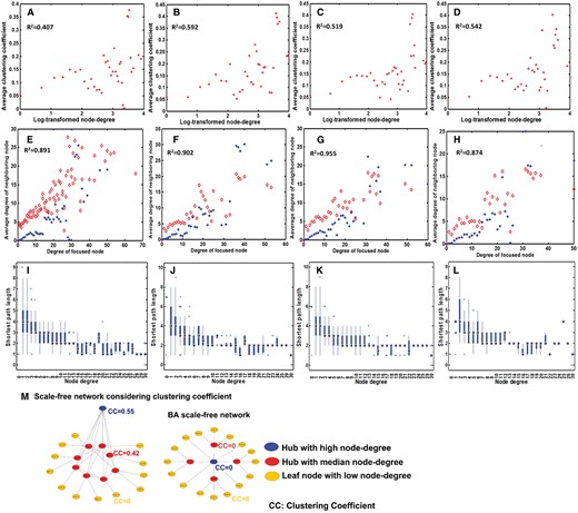
Clustering coefficient distribution revealing that each reaction network has one large, densely connected subnetwork. (A–D) The distribution of the clustering coefficient of the reaction network versus log-transformed node degree for E. coli K-12, K. pneumoniae MGH, S. enterica serovar and Y. pestis, respectively. (E–H) The degree of node versus the average degree of its neighbors in the reaction network (red dots) for each of the four species, along with blue dots representing the corresponding predicted average degree of the neighbors, where the x-axis represents all the nodes with a specific node degree, and the y-axis is the average node degree across all the corresponding neighboring nodes. (I–L) The node degree versus the average shortest path length of nodes with a specific degree for the four species. (M) A schematic illustration of a (simplified) reaction network versus a BA scale-free network.
By integrating the above analyses, we posit that reaction networks have the following organizing principles: (1) once currency metabolites, parallel and redundant reactions are simplified as the above, the resulting reaction networks each follow a power-law distribution by its node degree, and have its clustering coefficient positively correlated with the corresponding node degree (log-transformed); and (2) each resulting reaction network has exactly one large, densely connected subnetwork, which is derived from the clustering coefficient and shortest path lengths of the hub–nodes (Figure 4I–L and see ‘Materials and methods’ section).
Structural and functional characteristics of the reaction networks
We have conducted a clustering analysis of nodes in each reaction network based on the similarity of their shortest path lengths (see ‘Materials and methods’ section) and found that each of the 17 networks indeed has exactly one large densely connected core, providing evidence to our predicted organizing principle of reaction networks above.
The core accounts for 54–64% of the nodes in each of the 17 reaction networks. Removal of the core reactions from each network results in a sparsely connected subnetwork, referred to as the peripheral subnetwork. Further analyses revealed that this subnetwork naturally falls into two parts with one consisting of predominantly nutrient-uptake genes and catabolic enzymes and the other consisting of virtually all anabolic enzymes. These two modules are referred to as catabolic and anabolic module, respectively (Figure 5A). The catabolic and anabolic modules consist of 18–34% and 8–18% nodes of a network across the 17 networks, respectively (Supplementary Table S5). Furthermore, each peripheral module tends to form a largely linear structure with the edges of the catabolic module generally directed toward the core and edges of the anabolic module largely directed from the core. Figure 5B shows the detailed information regarding the directions and the structures of the two peripheral modules of E. coli.
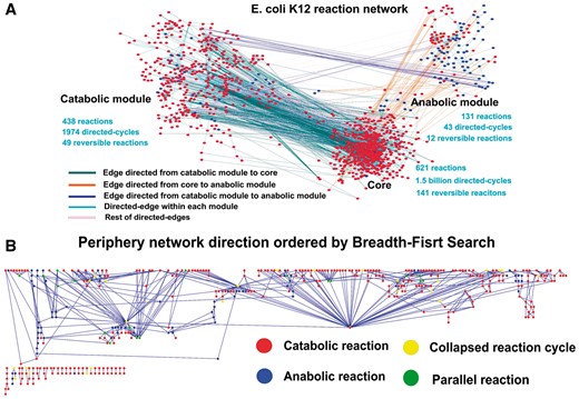
The structure of the reaction network for E. coli K12. (A) The reaction network for E. coli K-12 MG1655 consists of three subnetworks: the core, the catabolic and the anabolic modules, where the edges are color-coded according to the direction of each reaction linking two neighboring modules, and the nodes are also color-coded according to the reaction type, i.e. catabolic or anabolic reaction. (B) A layout of the peripheral module showing a layered structure from top down, where each simple reaction cycle is collapsed into one yellow node.
Detailed analyses revealed that each core consists of a large number of directed simple and short cycles, ranging from 0.03 to 11.2 billion across the 17 networks, compared with the simpler structures of the peripheral modules. Specifically, the average numbers of simple reaction cycles are ∼2000 in the peripheral modules versus ∼1.5 billion in the core, and the average number of reversible reactions in the core and the periphery are 142 and 61, respectively (paired t-test, P < 1.67E-17). In addition, among the enzymatic reactions, 24, 12 and 9% are reversible ones in the core, the catabolic and the anabolic modules, respectively. The enzymes in each core tend to enrich a similar set of metabolic functions across the 17 networks, for interconversion among a large variety of intermediate metabolites. In addition, the core metabolites tend to have smaller numbers of carbons than those in the peripheral modules, 17.45 versus 25.49 carbons per carbon-containing chain (paired t-test, P < 4.32E-10) (Supplementary Table S6), which is consistent with the functional roles of the three module types.
Metabolic fluxes in reaction networks
Here, we study how insights gained above can guide metabolic flux analyses. We focus our study on E. coli K12, as it has the most complete metabolic network and a large number of gene expression datasets collected under a variety of conditions.
Kinetic parameters of enzymes in the three subnetworks
We have examined the distributions of two important kinetic parameters: KM (Michaelis–Menten constant) and Kcat (turnover number) of enzymes plus Kcat/KM (enzyme efficiency) (see ‘Materials and methods’ section) in each of the three subnetworks. The average Kcat values are 522, 494 and 298 s−1 for the core, the catabolic and the anabolic modules [one-way analysis of variance (ANOVA), P < 0.023; n = 455], respectively, and the average KM values are 90, 100 and 114 µM−1 (one-way ANOVA, P < 0.014; n = 263), respectively. We also found that Kcat/KM values are considerably higher in the core than those in the peripheral modules (Supplementary Table S7), indicating that the reaction efficiency tends to be higher in the core than those in the peripheral modules, 1.5 and 3 times higher on average, respectively.
Characteristics of gene expression patterns in the three subnetworks
We have analyzed the gene expression data of E. coli K12 collected under 94 nutrient conditions, which are grouped into three nutrition levels: poor (M9 medium), medium (MOPS medium) and rich [Luria-Bertani (LB) broth] [35] (Supplementary Data S2), to examine how the gene expression profile of each subnetwork changes treated with the three nutrition levels.
For each nutrient level, we profiled the expression levels of genes in each subnetwork and analyzed the expression profiles of the core versus the peripherals using information entropy [36]. Specifically, the expression values of each sample within each module-specific gene set are considered as a distribution to estimate its information entropy (see ‘Materials and methods’ section). Hence, each of the three modules has an entropy value for each nutrient condition, and each data point in the three-dimension space of Figure 6A and B shows the three entropies of the three submodules for the E. coli metabolic network under each growth (nutrient) condition. The entropy values for the core form three distinct clusters corresponding to the three nutrient levels, while neither of the peripherals shows such specificity across three nutrient levels (Figure 6A and B and Supplementary Table S8). These results suggest that, on a global scale, the expression profiles of the core genes have identifiable states in response to nutrient changes, while the peripherial genes do not have this property.
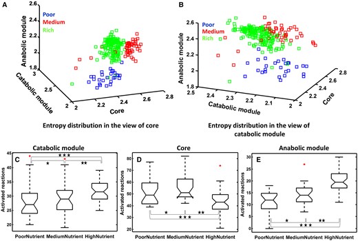
FBA and entropy of gene expression profiles. (A and B) Entropy distribution for gene expression profiles of the three subnetworks when treated with three types of nutrients. (A)The front view shows the nutrient-specific entropy distribution of genes in the core; the side view gives nutrient-specific entropy distribution of genes in the catabolic module; and the top view displays the nutrient-specific entropy distribution of genes in the anabolic module. (B) The three views are defined similarly but with catabolic genes in the front, core genes on the side and anabolic genes in the top. (C–E) Boxplots of the numbers of the activated reactions for the catabolic module (n = 41, one-way ANOVA, P < 9.18E-3; multiple comparison using Tukey's post hoc test, *P = 0.59 no significant, **P < 0.01 and ***P < 0.04), core (n = 41, one-way ANOVA, P < 6.52E-13; multiple comparison using Tukey's post hoc test, *P = 0.041, **P < 2.51E-5 and ***P < 1.7E-3) and anabolic module(n = 41, one-way ANOVA, P < 8.74E-10; multiple comparison using Tukey's post hoc test, *P = 0.012, **P < 0.01 and ***P < 1.3E-5), when treated with three different types of nutrient.
Metabolic flux patterns with different nutrients
We have also examined how the metabolic fluxes, calculated using FBA to maximize the growth rate, change across different nutrition levels in the three subnetworks (see ‘Materials and methods’ section). Nonzero flux reactions are identified using FBA (the COBRA Toolbox [37]), which maximize the growth rate. As shown in Figure 6C–E, the total number of nonzero flux reactions in the core goes down as the nutrition level goes up. In contrast, the number of nonzero flux reactions in each peripheral module goes up with the increasing level of nutrition (Supplementary Table S9).
These observations suggest: there may exist a relatively stable pool of precursors for macromolecular syntheses and cell division. Specifically, the number of precursors needed to be synthesized in the core goes down as the nutrition level goes up, namely, the nutrient contains more precursor molecules. In comparison, the activities in the catabolic module go up as the composition of the richer nutrient becomes more complex. For the anabolic module, its increased activity level with the increasing nutrition level reflects the increased overall activity of the host cells, including metabolic activities enabled by the increased supplies of the basic building blocks and energy.
Further support for the above proposition comes from metabolites present in the three subnetworks across the three conditions. We noted that all the 272 metabolites synthesized in the core under the rich nutrient are a subset of all the 354 metabolites synthesized under the poor nutrient, which are derived based on the nonzero flux reactions. Out of the synthesized metabolites under the poor nutrient, 12 are condition-specific precursor metabolites directly used by the anabolic module for macromolecular syntheses (Supplementary Table S10).
Based on the above analyses, we conclude: the peripheral modules can sense and respond to changes in the environment by altering their gene expression patterns and metabolic fluxes, while the core seems to play a buffering role to maintain their overall expression levels stable and adjust their reactions to compensate for what the nutrient does not provide in support of cell growth and housekeeping. Overall, metabolic fluxes go from one end of the catabolic module to the other, and then enter the core where substantial synthesis activities will take place to produce precursors needed for macromolecular synthesis in the anabolic module.
Materials and methods
Metabolic networks
Genome-scale microbial metabolic networks were obtained from the BIGG database [38]. The following criteria are used in our selection: for each species in BIGG, we selected one most complete metabolic network, which gives rise to 17 metabolic networks of 17 species. Table 2 gives the list of the names of the organisms along with the relevant information of each network.
Information of 17 metabolic networks used in this study
| Organism | BIGG ID | #Metabolites | #Reactions | #Genes |
|---|---|---|---|---|
| Bacillus subtilis 168 | iYO844 | 991 | 1250 | 844 |
| Clostridium ljungdahlii DSM 13528 | iHN637 | 698 | 785 | 637 |
| Escherichia coli K-12 MG1655 | iAF1260 | 1688 | 2382 | 1261 |
| Geobacter metallireducens GS-15 | iAF987 | 1109 | 1285 | 987 |
| Helicobacter pylori 26695 | iIT341 | 485 | 554 | 339 |
| Klebsiella pneumoniae MGH 78578 | iYL1228 | 1658 | 2262 | 1229 |
| Methanosarcina barkeri Fusaro | iAF692 | 628 | 690 | 692 |
| Pseudomonas putida KT2440 | iJN746 | 909 | 1056 | 746 |
| Saccharomyces cerevisiae S288c | iMM904 | 1226 | 1577 | 905 |
| Salmonella enterica serovar Typhimurium | STM_v1_0 | 1800 | 2545 | 1271 |
| Shigella boydii CDC 3083-94 | iSbBS512_1146 | 1912 | 2592 | 1147 |
| Shigella dysenteriae Sd197 | iSDY_1059 | 1890 | 2540 | 1059 |
| Shigella flexneri 2a 2457T | iS_1188 | 1914 | 2620 | 1188 |
| Shigella flexneri 5 8401 | iSFV_1184 | 1917 | 2622 | 1184 |
| Staphylococcus aureus N315 | iSB619 | 655 | 743 | 619 |
| Thermotoga maritima MSB8 | iLJ478 | 570 | 652 | 482 |
| Yersinia pestis CO92 | iPC815 | 1552 | 1961 | 815 |
Construction of a reaction network
For each retrieved metabolic network, we constructed a reaction network using a well-established procedure [9]. Specifically, each reaction in the target metabolic network is represented as a node and each metabolite as an edge. Each edge connects two reaction-representing nodes with its direction going from a metabolite-producing reaction to a metabolite-consuming reaction.
Simplification of metabolic networks
In total, 28 such molecular species, for the simplicity of discussion, all referred to as currency metabolites, are removed from our structural analysis: ACP, ADP, ATP, AMP, cMP, CO2, COA, CTP, FADH2, Fe2+, GMP, GDP, GTP, H+, H2O, MQN8, MQL8, NAD, NADH, NADP, NADPH, O2, Pi, PPI, Q8, Q8H2, UDP and UMP.
Network parameters
Merging parallel reactions
Enzymes are classified into four groups based on the numbers of homologs and component proteins (monomeric or multimeric enzyme) that an enzyme has encoded in the host genome: (1) monomeric enzymes without homologs, denoted as GE; (2) monomeric enzymes with at least one homolog, termed MHGE; (3) multimeric enzymes without homolog, marked as MSGE; and (4) multimeric enzymes with at least one homolog, named MHSGE. We noted that each GE or MHGE enzyme catalyzes more reactions than each MSGE or MHSGE enzyme on average (Figure 2A–D and Supplementary Figure S4; and Supplementary Table S3), where the GE and MHGE enzymes are identified based on [33], and the reactions catalyzed by such enzymes tend to have similar substrates or products, called parallel reactions. To remove redundant information because of parallel reactions, each group of parallel reactions is collapsed into one reaction by combining the substrates on one side of the reaction and the products on the other side (Supplementary Figure S1B).
Eliminating redundant edges
Consider any two consecutive reversible reactions with one using the products of the other one as the substrates, which may result in redundant edges when constructing a reaction network, namely: if the product of a reaction is the substrate of another reaction, then an edge directing from the first reaction to the second will be included in the reaction network. An example of such a case is shown in Supplementary Figure S1C, along with how such redundant edges are removed.
Estimating the level of network completeness and implication to topological parameter estimation
We have assessed the level of completeness of each given metabolic network using four parameters of the network: the numbers of metabolites, reactions, metabolic genes and all genes encoded in the host genome. We have observed that (i) the smaller the ratio between the number of metabolites and the number of reactions , the more complete the network, the higher the exponent value in the power-law distribution of the network’s node degrees and the smaller the clustering coefficient will be; and (ii) the same holds for the three above properties with the increase of the ratio between the number of metabolic genes and the total number of genes encoded in the genome.
To ensure that the above observation is statistically sound, we conducted a sampling analysis of the E. coli K12 network (E. coli iAF1260), one of the most complete metabolic network among all known such networks, to examine if the above observations are indeed correct, when some portions of the network are randomly removed. Specifically, our sampling process aims to mimic the following insight gained through increasingly complete models of E. coli. A few distinct metabolic subsystems have been identified and integrated into E. coli metabolic models at different times, namely, the e_coli_core, iJR904, iAF1260 and iJO1366 models, each of them being more complete than the preceding one(s), according to the identified complementary subsystems, i.e. the central metabolism, the biosynthesis reactions (amino acid metabolism and nucleotide metabolism), exchange reactions and species-specific reactions [40–42], respectively.
We have conducted a simulation analysis by randomly removing reactions from the network but with different probabilities for reactions in the different subsystems defined above. Specifically, the exchange reactions and biosynthesis reactions were given higher probabilities than the reactions in the central metabolism. A roulette-wheel method was used to select reactions for removal [43]. Supplementary Figure S7 shows the detailed information of the sampled networks of the E. coli iAF1260 model and the associated predictions of the two topological parameters. From the figure, we can see that our observation is correct.
The first model achieves an average = 0.695 ( statistic 19.21 and P < 1.0E-4), and the second model achieves an average = 0.628 ( statistic 18.35 and P < 6.0E-4) across the 17 networks.
The average degree of neighboring nodes derived from the clustering coefficients
Inference of a unique large and dense subnetwork
We assume, without loss of generality, that there are two independent giant components, which have the same topology and size in this reaction network; hence, the largest hub node in each giant component has neighboring nodes with an average node degree . This result means that there are 2 nodes with an average degree or larger for the given reaction network including two independent giant components, in other words, the average degree of the top 2 largest-degree nodes should be larger than for this reaction network, which is the necessary condition to form two independent giant components, and we know the number of nodes with an average node degree is monotonously exponential decreased along with the increment of in a scale-free network, so the question of whether existing two independent giant components in a reaction network is converted as whether the average node degree of the top 2 largest-degree nodes is larger than the expected node degree to form two independent giant components. Systematic examination of all the 17 reaction networks be given in Supplementary Table 13 and revealed that almost of reaction networks are satisfied the inequation of .
Furthermore, we noted that the shortest-path length for individual nodes tends to decrease rapidly with the increase of the node degrees across all 17 networks, and the distance (the number of edges) between any hub–node and any of its leaf node is most 4. Under the assumption that all hub–nodes are reachable by directed pathways (Figure 4I–L and Supplementary Figure S9), we can show that each network has one large (covering at least 25%) dense subnetwork. Supplementary Figure S10 provides additional information in support of this assumption.
Identifying metabolic network modules
We conducted a hierarchical clustering analysis of nodes in each of 17 reaction networks based on the similarity derived from the shortest-path lengths [45], as we have inferred there is a unique large and dense subnetwork in each metabolic network in the last section. We found that that hub–nodes tend to connect with each other, and the short path lengths between the hub–nodes are small (<4 for most metabolic networks) (Supplementary Figure S9). So, the core module of metabolic network can be identified as follows: the similarity measures for the clustering analysis are considered as the shortest-path lengths, and the distance criterion for splitting the hierarchical clustering tree was set to. Then, removal of the core structure from each reaction network leads to two substantially connected substructures, as most of the upstream nodes of the remaining subnetwork are catabolic reactions, and almost all downstream nodes are anabolic reactions based on the topological order of the remaining subnetwork. Therefore, we have three subnetworks, which correspond to the three well-known modules of metabolic networks.
Kinetic parameters of E. coli K12 enzymes
Kinetic rate constants KM and Kcat for each enzyme in E. coli K12 are collected from the Brenda database under the normal growth condition [46], i.e. no mutation, pH 7.0 and 37°C. Missing data are further collected from the EcoCyc database [47]. Overall, 1049 enzymes have KM values and 638 have Kcat values (Supplementary Data S3).
Gene expression data for E. coli K12
Gene expression data for E. coli K12 are retrieved from the M3D database [35]. Specifically, data were collected on E. coli K12 in exponential growth with pH 7.0, 37°C and aerobically in three nutrients: M9, MOPS and LB, totaling 27, 27 and 40 samples for the three nutrient types, respectively.
Entropy-based state analysis
FBA under a given condition
Statistical analyses
Statistical analysis was carried out using Matlab R2014a. ANOVA was used to identify significant variance of data set with multiple samples. P-value 0.05 was used as the cutoff in selecting a statistical significant test.
Data availability
The Matlab codes used to conduct all the analyses in this study, along with all the data used and generated are available at: https://github.com/lgyzngc/metabolic-network-analysis.
Discussion
While substantial amount of work has been conducted in both structural and functional analyses of metabolic networks, there is a clear disconnection between the two [48–50]. Consequently, different and sometimes conflicting results have been derived regarding the fundamental properties of metabolic networks, depending on specific representation schemes [22, 24, 25].
Our discovery that microbial reaction networks, after simplification of certain nonessential elements, follow a power-law distribution by their node degree and have positive correlation between their clustering coefficient and the corresponding node degree (after log-transformation) in the same network has led to an important realization: (microbial) reaction networks each consist of one large, densely connected core plus two peripheral modules: one responsible for breaking down nutrients to basic metabolites and one for macromolecular syntheses from a set of possibly predefined precursors. This is derived through an application of the topological properties of metabolic networks, which confirms the previously observed bow tie structure of metabolic networks [26, 51]. It should be noted that the bow tie structure of metabolic networks was proposed only as a preliminary concept to explain the functional modules of metabolic network. All the implementation was derived from manual yet small- or local-scale precise annotation of metabolic system or functional analysis of metabolic pathways, rather than using the topological properties of metabolic network. To our knowledge, this is the first genome-scale functional compatibility model of structure decomposition of microbial metabolic networks by inferring the topological organizing principles.
Functional analyses of the three subnetworks led to the discovery that both peripheral modules have simple, layered structures with a clear flux directionality, while for the core, the flux directionality is nutrient-dependent, as many of the reactions in the core are reversible and/or form reaction cycles. Based on our results, we posit that (i) the core synthesizes a set of precursors used for macromolecule synthesis by the anabolic module; and (ii) it is the insufficient precursors needed for cell division, in the nutrient that determine the directionalities of many of the reversible reactions in the core [52], i.e. the core is driven to synthesize all the insufficient precursors needed for cell growth and division.
Our model is consistent with a number of recent large-scale metabolomic studies of E. coli. In a study that has reported 3800+ mutants of E. coli each having one deletion of a distinct gene and intracellular concentrations of 7000+ metabolites in each mutant, the authors reported that concentrations of most metabolites produced by the core subnetwork (consisting of the pentose phosphate pathway, TCA cycle, nucleotide salvage pathway, oxidative phosphorylation, nitrogen metabolism among a few other essential pathways) are stable against the gene deletions of the corresponding pathway, while the concentrations of metabolites in the amino acid metabolism, which fall into the anabolic subnetwork in our analyses, tend to change with deletion of the genes of the relevant pathway [53]. This is clearly consistent with our model and prediction. A study recently reported that during the growing phase, the intracellular concentrations of ∼67% of metabolites in E. coli are equal to or larger than the values of the relevant enzymes [54], and the enzyme expression levels of the carbohydrate metabolism (as part of our core) decrease with the increase of the growth rate, while enzyme expression levels in the amino acid biosynthesis (anabolic module) have the opposite behavior [55]. Those observations are consistent with our prediction.
The above analyses may explain two puzzling issues: (1) why the number of elementary flux modes is so large to be practically solvable for any sizeable metabolic networks [12]; and (2) why FBAs generally do not produce accurate estimates of the actual fluxes in a metabolic system, as such analyses generally do not take into consideration the nonlinear topology of core constituents of the reaction cycles and reversible reactions and the gap between what the nutrients offer and what are needed for cell growth and division. For example, the tricarboxylic acid (TCA) cycle, which provides electrons to the respiratory chain for energy production and precursor metabolites for macromolecule biosynthesis, is a self-balancing reaction cycle in terms of its substrates. Hence, its reactions should have large flux. However, maximizing the growth rates of an organism may tend to assign zero-fluxes to some TCA reactions by FBA if it does not constrain the amount and types of the substrates into the TCA cycle, as such metabolites can be supplied from the extracellular environment or other pathways [56].
The new insights gained in this study can not only explain puzzling issues as shown above but also provide useful guiding information for strain optimization needed for bioengineering. For example, in a recent study, four metabolic reactions for the synthesis of cytosolic acetyl-coA in Saccharomyces cerevisiae were integrated by inserting the genes into the genome, so that they become part of the central carbon metabolism [30].
We anticipate that this study will lead to new types of structural and functional analyses of metabolic networks through considering both structure and function of a metabolic network at the same time, hence possibly leading to more reliable and more useful network topology-related analyses. It is noteworthy that the predicted metabolic network models may be still potentially incomplete, as the complete metabolic pathways have not been fully elucidated experimentally, so the experimental validation for the inferred network parameters is a further improvement of this work.
The inconsistencies regarding properties of the reaction networks as reported by different authors are largely because of improper representations of different components of a network as well as because of the incompleteness of the reaction networks studied.
Our analyses revealed that each of the reaction networks studied here can be naturally decomposed into three subnetworks each with specific biological functions and structural characteristics: a core covering majority of the enzymatic reactions encoded in the host genome and having highly interconnected edges, which provide robustness of the core, and two sparsely connected subnetworks, one mainly responsible for catabolic reactions and the other for anabolic reactions.
Metabolic fluxes generally go from the catabolic subnetwork to the core where substantial interconversions occur with the flux directions determined by nutrients, and then to the anabolic subnetwork.
Each subnetwork has a distinct set of enzyme kinetic parameters highly consistent with its designed functions.
Our structural and functional predictions of metabolic networks are supported by gene expression data under growth conditions of E. coli. Such models can inform pathogenic metabolomics and systems biological studies.
Acknowledgements
The authors thank Dr Wei Du at Jilin University for helpful discussion of the manuscript
Funding
This work was supported by the US Department of Energy BioEnergy Science Center (grant number DE-PS02-06ER64304).
Gaoyang Li is a PhD student in the College of Computer Science and Technology at Jilin University, China. This work was conducted when he was a visiting student at Ying Xu’s lab at the University of Georgia. His research interests include computational systems biology, metabolomics and metabolic dynamic optimization.
Huansheng Cao was a postdoctoral researcher in the Department of Biochemistry and Molecular Biology and Institute of Bioinformatics at the University of Georgia. His interests include microbial systems biology and microbiome research. He is now an assistant research professor in the Biodesign Institute of Arizona State University.
Ying Xu is a Regents-GRA Eminent Scholar Chair and Professor in the Department of Biochemistry and Molecular Biology and Institute of Bioinformatics at the University of Georgia. His interests include computational systems biology of cancer and bacteria.
References
Author notes
Gaoyang Li and Huansheng Cao contributed equally.
