


Abstract
Linkage analysis has played an important role in understanding genome structure and evolution. However, two-point linkage analysis widely used for genetic map construction can rarely chart a detailed picture of genome organization because it fails to identify the dependence of crossovers distributed along the length of a chromosome, a phenomenon known as crossover interference. Multi-point analysis, proven to be more advantageous in gene ordering and genetic distance estimation for dominant markers than two-point analysis, is equipped with a capacity to discern and quantify crossover interference. Here, we review a statistical model for four-point analysis, which, beyond three-point analysis, can characterize crossover interference that takes place not only between two adjacent chromosomal intervals, but also over multiple successive intervals. This procedure provides an analytical tool to elucidate the detailed landscape of crossover interference over the genome and further infer the evolution of genome structure and organization.
Introduction
Linkage, a phenomenon by which adjacent genes on the same chromosomal region tend to be inherited together, has been extensively investigated since its first discovery by several pioneering geneticists [1]. By measuring the frequency with which a single chromosomal crossover (chiasmata) takes place between two genes during meiosis, known as the recombination fraction, linkage analysis has served as a primary tool of gene localization and ordering. The past several decades have seen the tremendous application of linkage analysis to mapping and identifying causal genes that affect Mendelian diseases or quantitative traits [2–5]. Although linkage mapping was largely replaced by genome-wide association studies during the past few years, its potential to identify genes involved in disease etiology has been recognized and reactivated by the increasing availability of family-based exome and whole-genome sequence data [6, 7]. Apart from its application for gene mapping, linkage analysis has been instrumental for comparative analysis of genome structure and organization from which the evolution of sexually reproducing organisms in response to environmental changes can be inferred [8]. For example, heterochiasmy, i.e. differences between female and male recombination fractions, regarded as an important evolutionary force shaping the nucleotide landscape of sex-specific genomes, can well be studied through linkage analysis [9].
Two-point analysis is the most basic approach for linkage analysis and has been extended to multi-point analysis that analyzes information from many markers simultaneously [2, 4]. Multi-point analysis has been widely used to construct genetic linkage maps that describe the frequency and distribution of meiotic crossovers along a chromosome within a population. However, traditional multi-point analysis ignores crossover interference [4], although the assumption may not conform to the actual existence of interference. As a phenomenon by which the occurrence of one crossing-over interferes with the coincident occurrence of another crossing-over in the same pair of chromosomes [10], crossover interference has been recognized to play a more important role in evolution and speciation than previously appreciated [11–18]. A new three-point analysis that analyzes simultaneously the linkage relationship among three adjacent markers has been developed to estimate the magnitude and distribution of crossover interference along a chromosome [19–21]. This approach can also improve the gene ordering and the estimation precision of linkage for dominant-inherited markers [22], and it has been modified to accommodate the different types of populations including controlled crosses [22], natural human family populations [23] and open-pollinated plant populations [24, 25].
Three-point analysis has an adequate degree of freedom that allows it not to rely on the hypothesis that the recombination events between two adjacent marker intervals are independent, thus providing a possibility to estimate crossover interference [26, 27]. Nevertheless, it is possible that interference occurs simultaneously between more than two marker intervals in marker-dense chromosomal regions to form high-order crossover interference (Figure 1). Despite its importance, this issue has not been reviewed and assessed in the literature. In this article, we argue that well-developed three-point analysis can be extended to perform linkage analysis using more than three markers. Such an extension opens an avenue to estimate and test crossover interference that may take place along multiple intervals across a chromosome. We show that four-point analysis can not only preserve the statistical properties of parameter estimation characteristic of two- and three-point analysis, but also provide additional information about how multiple marker intervals interfere with each other to affect genome structure.
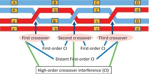
Diagram of the occurrence of crossover interference (CI) of different orders among markers A–D over a chromosome.
Four-point analysis for the backcross
Estimation
Suppose there is a backcross mapping population of n progeny in which a suite of molecular markers was generated. Consider four-order markers, A-B-C-D, with alleles A versus a, B versus b, C versus c and D versus d, respectively. Thus, backcross ABCD/abcd × abcd/abcd generates 16 marker genotypes in the progeny, each exactly corresponding to its gamete genotype contributed by the heterozygote F1. During meiosis, two homologous chromosomes of the F1 each duplicate into sister chromatids that crossover between markers A and B (first crossover), between markers B and C (second crossover) and between markers C and D (third crossover) (Figure 1). Crossover interference may occur if the occurrence of one crossover affects the occurrence of other crossovers nearby. In this four-marker case, crossover interference takes place between the first and the second crossover, between the second and the third crossover, between the first and the third crossover and jointly among the three crossovers. The first two crossover interferences have been explored in the genetic literature, but we are ignorant of the last two. Four-point analysis can reveal these two unexplored types of crossover interference.
Eight gamete types and their frequencies at four ordered markers A-B-C-D produced by the heterozygous F1 parent in a backcross population of n progeny, along with observations of each genotype
| No. | Gamete type | Number of crossovers | Gamete typeFrequency | Diplotype | Genotype | Observation | ||
|---|---|---|---|---|---|---|---|---|
| A-B | B-C | C-D | ||||||
| 1 | ABCD | 0 | 0 | 0 | g000 | ABCD|abcd | AaBbCcDd | n1111 |
| abcd | abcd|abcd | aabbccdd | n0000 | |||||
| 2 | ABCd | 0 | 0 | 1 | g001 | ABCd|abcd | AaBbCcdd | n1110 |
| abcD | abcD|abcd | aabbccDd | n0001 | |||||
| 3 | ABcd | 0 | 1 | 0 | g010 | ABcd|abcd | AaBbccdd | n1100 |
| abCD | abCD|abcd | aabbCcDd | n0011 | |||||
| 4 | ABcD | 0 | 1 | 1 | g011 | ABcD|abcd | AaBbccDd | n1101 |
| abCd | abCd|abcd | aabbCcdd | n0010 | |||||
| 5 | Abcd | 1 | 0 | 0 | g100 | Abcd|abcd | Aabbccdd | n1000 |
| aBCD | aBCD|abcd | aaBbCcDd | n0111 | |||||
| 6 | AbcD | 1 | 0 | 1 | g101 | AbcD|abcd | AabbccDd | n1001 |
| aBCd | aBCd|abcd | aaBbCcdd | n0110 | |||||
| 7 | AbCD | 1 | 1 | 0 | g110 | AbCD|abcd | AabbCcDd | n1011 |
| aBcd | aBcd|abcd | aaBbccdd | n0100 | |||||
| 8 | AbCd | 1 | 1 | 1 | g111 | AbCd|abcd | AabbCcdd | n1010 |
| aBcD | aBcD|abcd | aaBbccDd | n0101 | |||||
Gametes ABCD and abcd:there are no crossovers for each pair,
Gametes ABCd and abcD: there is only a crossover from the third pair,
Gametes ABcd and abCD: there is only a crossover from the second pair,
Gametes ABcD and abCd: there are crossovers from the second and third pair,
Gametes Abcd and aBCD: there is only a crossover from the first pair,
Gametes AbcD and aBCd: there are crossovers from the first and third pair,
Gametes AbCD and aBcd: there are crossovers from the first and second pair,
Gametes AbCd and aBcD: there are crossovers for each pair.
Hypothesis tests
Evaluation by computer simulation
Table 2 gives the results about parameter estimation by four-point analysis. In general, the recombination fractions can be reasonably well estimated for a moderate sample size (n = 200), regardless of the degree of linkage and crossover interference. Notably, the estimation of low-order crossover interference can be well estimated with a moderate sample size, but the estimation precision of high-order crossover interference hinges more strongly on sample size. A large sample size (n = 400) is needed to obtain precise estimation of high-order crossover interference. The estimation of the recombination fraction is not affected by the occurrence of crossover interference (Table 2); that is, the linkage can be well estimated, regardless of whether there is a crossover interference.
Simulation results under different scenarios of occurrence of high-order crossover interference for a backcross of different sample sizes estimated by four-point analysis, in comparison with those by two- and three-point analysis. The standard errors of parameter estimates are given in parentheses
| Scenario 1 | Scenario 2 | Scenario 3 | |||||||
|---|---|---|---|---|---|---|---|---|---|
| Methods | True | n = 200 | n = 400 | True | n = 200 | n = 400 | True | n = 200 | n = 400 |
| Four-point Analysis | |||||||||
| rAB | 0.05 | 0.041(0.013) | 0.042(0.099) | 0.05 | 0.051(0.016) | 0.049(0.009) | 0.05 | 0.044(0.014) | 0.046(0.010) |
| rBC | 0.15 | 0.155(0.026) | 0.157(0.016) | 0.15 | 0.146(0.024) | 0.152(0.017) | 0.15 | 0.154(0.024) | 0.149(0.019) |
| rCD | 0.3 | 0.309(0.030) | 0.302(0.021) | 0.3 | 0.302(0.038) | 0.300(0.025) | 0.3 | 0.302(0.038) | 0.300(0.020) |
| rAC | 0.17 | 0.165(0.026) | 0.169(0.019) | 0.17 | 0.168(0.027) | 0.171(0.018) | 0.17 | 0.170(0.025) | 0.162(0.020) |
| rBD | 0.45 | 0.455(0.033) | 0.450(0.025) | 0.45 | 0.449(0.040) | 0.453(0.025) | 0.45 | 0.452(0.038) | 0.443(0.024) |
| rAD | 0.458 | 0.453(0.034) | 0.449(0.024) | 0.44 | 0.438(0.041) | 0.442(0.026) | 0.449 | 0.445(0.040) | 0.436(0.023) |
| C1 | 2 | 2.455(1.141) | 2.301(0.818) | 2 | 2.040(1.087) | 2.042(0.694) | 2 | 2.080(1.140) | 2.367(0.755) |
| C2 | 0 | 0.091(0.100) | 0.093(0.066) | 0 | 0.000(0.000) | 0.000(0.000) | 0 | 0.041(0.060) | 0.065(0.058) |
| C3 | 1 | 1.218(0.564) | 1.217(0.388) | 1 | 1.084(0.493) | 1.003(0.347) | 1 | 1.154(0.605) | 1.169(0.395) |
| C4 | 2 | 2.390(2.746) | 2.161(1.405) | 0 | 0.000(0.000) | 0.000(0.000) | 1 | 0.934(1.442) | 1.425(1.283) |
| Two-point Analysis | |||||||||
| rAB | 0.05 | 0.039(0.014) | 0.043(0.011) | 0.05 | 0.048(0.017) | 0.048(0.010) | 0.05 | 0.047(0.016) | 0.043(0.011) |
| rBC | 0.15 | 0.146(0.024) | 0.155(0.019) | 0.15 | 0.152(0.025) | 0.150(0.018) | 0.15 | 0.152(0.024) | 0.150(0.018) |
| rCD | 0.3 | 0.306(0.037) | 0.302(0.023) | 0.3 | 0.301(0.033) | 0.300(0.024) | 0.3 | 0.305(0.036) | 0.300(0.021) |
| rAC | 0.17 | 0.158(0.026) | 0.166(0.021) | 0.17 | 0.172(0.026) | 0.170(0.019) | 0.17 | 0.170(0.026) | 0.165(0.017) |
| rBD | 0.45 | 0.443(0.039) | 0.448(0.027) | 0.45 | 0.453(0.035) | 0.446(0.026) | 0.45 | 0.453(0.039) | 0.444(0.025) |
| rAD | 0.458 | 0.444(0.040) | 0.446(0.028) | 0.44 | 0.443(0.035) | 0.437(0.026) | 0.449 | 0.447(0.038) | 0.437(0.025) |
| C1 | 2 | – | – | 2 | – | – | 2 | – | – |
| C2 | 0 | – | – | 0 | – | – | 0 | – | – |
| C3 | 1 | – | – | 1 | – | – | 1 | – | – |
| C4 | 2 | – | – | 0 | – | – | 1 | – | – |
| Three-point Analysis | |||||||||
| rAB | 0.05 | 0.043(0.016) | 0.041(0.010) | 0.05 | 0.049(0.016) | 0.052(0.012) | 0.05 | 0.044(0.014) | 0.048(0.011) |
| rBC | 0.15 | 0.147(0.021) | 0.154(0.018) | 0.15 | 0.151(0.026) | 0.152(0.019) | 0.15 | 0.156(0.024) | 0.152(0.016) |
| rCD | 0.3 | 0.307(0.031) | 0.300(0.024) | 0.3 | 0.300(0.034) | 0.298(0.022) | 0.3 | 0.300(0.032) | 0.297(0.023) |
| rAC | 0.17 | 0.158(0.025) | 0.164(0.019) | 0.17 | 0.172(0.027) | 0.172(0.021) | 0.17 | 0.170(0.024) | 0.168(0.019) |
| rBD | 0.45 | 0.444(0.034) | 0.444(0.026) | 0.45 | 0.447(0.038) | 0.450(0.024) | 0.45 | 0.448(0.031) | 0.445(0.025) |
| rAD | 0.458 | 0.445(0.033) | 0.444(0.025) | 0.44 | 0.437(0.038) | 0.440(0.025) | 0.449 | 0.442(0.031) | 0.438(0.025) |
| C1 | 2 | – | – | 2 | – | – | 2 | – | – |
| C2 | 0 | – | – | 0 | – | – | 0 | – | – |
| C3 | 1 | – | – | 1 | – | – | 1 | – | – |
| C4 | 2 | – | – | 0 | – | – | 1 | – | – |
The simulated marker data were further analyzed by two- and three-point analysis. It can be seen that these approaches can also provide good estimates of the recombination fractions (Table 2), again suggesting that crossover interference does not affect the identification of linkage by two- or three-point analysis. The power of linkage analysis has been investigated previously (Lu et al. 2004). Here, we focus on the power analysis of detecting crossover interference, which is based on hypothesis tests of Equations (7a)–(7d). In general, the power of detecting low-order crossover interference (C1, C2 or C3) is high, reaching 0.95 or higher, even with a moderate sample size. However, to detect high-order crossover interference (C4), a larger sample size, such as 400, is needed.
For those unsequenced genomes, we do not know the order of their genes. However, gene order can be inferred from genotypic data. We performed simulation studies based on the above scenario to examine the power of gene ordering by four-point analysis. For a given set of markers, we considered all possible orders under each of which the likelihood of observations is calculated. The maximum likelihood corresponds to a most likely gene order. We found that four-point analysis can provide full power to correctly detect the optimal gene order with a moderate sample size (n = 200). Such power decreases slightly for three- and two-point analysis (Table 3). With a large sample size (n = 400), all approaches give full power. Compared with two-point analysis, the computing time of three- and four-point analysis is 1.5 and 2.5 times more, respectively.
Empirical power of correctly detecting an optimal order of genes with varying recombination fractions and interference degrees under different sample sizes
| Methods | n = 200 | n = 400 |
|---|---|---|
| Two-point analysis | 98% | 100% |
| Three-point analysis | 99% | 100% |
| Four-point analysis | 100% | 100% |
| Methods | n = 200 | n = 400 |
|---|---|---|
| Two-point analysis | 98% | 100% |
| Three-point analysis | 99% | 100% |
| Four-point analysis | 100% | 100% |
Four-point analysis for a full-sib family: a mixture model
The backcross is the simplest design for linkage analysis that contains a full amount of marker segregation information. For the backcross, we can derive explicit estimators for the linkage and the genetic interference. However, for more complex designs, such as the F2, in which genotypes may not be consistent with diplotype, a more sophisticated expectation-maximization (EM) algorithm should be implemented. Two heterozygous F1, ABCD/abcd × ABCD/abcd, are crossed to generate a segregating F2 population. Here, each F1 parent generates 16 gametes, which are divided into eight types (Table 1). Their cross generates 136 diplotypes collapsed into 81 distinguishable genotypes. Table 3 provides the genotype frequencies of the F2 progeny expressed in terms of products of gamete-type frequencies from the two heterozygous parents. It can be seen that the frequencies of heterozygous genotypes at two or more markers are a mix of products of gamete-type frequencies.
Four-marker genotype observations and expected frequencies composed of gamete-type frequencies produced by each parent in an F2 population. The expected numbers of each gamete type within each genotype are also given
| CCDD | CCDd | CCdd | CcDD | CcDd | Ccdd | ccDD | ccDd | ccdd | ||
|---|---|---|---|---|---|---|---|---|---|---|
| AABB | Frequency | g0002 | 2g000g001 | g0012 | 2g000g011 | 2(g000g010+g001g011) | 2g001g010 | g0112 | 2g011g010 | g0102 |
| Observation | n2222 | n2221 | n2220 | n2212 | n2211 | n2210 | n2202 | n2201 | n2200 | |
| g000 | 2 | 1 | 0 | 1 | φ3 | 0 | 0 | 0 | 0 | |
| g001 | 0 | 1 | 2 | 0 | 1-φ3 | 1 | 0 | 0 | 0 | |
| g010 | 0 | 0 | 0 | 0 | φ3 | 1 | 0 | 1 | 2 | |
| g011 | 0 | 0 | 0 | 1 | 1-φ3 | 0 | 2 | 1 | 0 | |
| g100 | 0 | 0 | 0 | 0 | 0 | 0 | 0 | 0 | 0 | |
| g101 | 0 | 0 | 0 | 0 | 0 | 0 | 0 | 0 | 0 | |
| g110 | 0 | 0 | 0 | 0 | 0 | 0 | 0 | 0 | 0 | |
| g111 | 0 | 0 | 0 | 0 | 0 | 0 | 0 | 0 | 0 | |
| AABb | Frequency | 2g000g110 | 2(g000g111+g001g110) | 2g001g111 | 2(g000g101+g011g110) | 2(g000g100+g001g101+ g010g110+g011g111) | 2(g001g100+g010g111) | 2g011g101 | 2(g010g101 + 2g011g100) | 2g010g100 |
| Observation | n2122 | n2121 | n2120 | n2112 | n2111 | n2110 | n2102 | n2101 | n2100 | |
| g000 | 1 | φ10 | 0 | φ7 | φ6 | 0 | 0 | 0 | 0 | |
| g001 | 0 | 1-φ10 | 1 | 0 | φ16 | φ15 | 0 | 0 | 0 | |
| g010 | 0 | 0 | 0 | 0 | φ23 | 1-φ15 | 0 | φ22 | 1 | |
| g011 | 0 | 0 | 0 | 1-φ7 | φ27 | 0 | 1 | 1-φ22 | 0 | |
| g100 | 0 | 0 | 0 | 0 | φ6 | φ15 | 0 | 1-φ22 | 1 | |
| g101 | 0 | 0 | 0 | φ7 | φ16 | 0 | 1 | φ22 | 0 | |
| g110 | 1 | 1-φ10 | 0 | 1-φ7 | φ23 | 0 | 0 | 0 | 0 | |
| g111 | 0 | φ10 | 1 | 0 | φ27 | 1-φ15 | 0 | 0 | 0 | |
| AAbb | Frequency | g1102 | 2g110g111 | g1112 | 2g011g101 | 2(g110g100+g111g101) | 2g111g100 | g1012 | 2g101g100 | g1002 |
| Observation | n2022 | n2021 | n2020 | n2012 | n2011 | n2010 | n2002 | n2001 | n2000 | |
| g000 | 0 | 0 | 0 | 0 | 0 | 0 | 0 | 0 | 0 | |
| g001 | 0 | 0 | 0 | 0 | 0 | 0 | 0 | 0 | 0 | |
| g010 | 0 | 0 | 0 | 0 | 0 | 0 | 0 | 0 | 0 | |
| g011 | 0 | 0 | 0 | 0 | 0 | 0 | 0 | 0 | 0 | |
| g100 | 0 | 0 | 0 | 0 | φ30 | 1 | 0 | 1 | 2 | |
| g101 | 0 | 0 | 0 | 1 | 1-φ30 | 0 | 2 | 1 | 0 | |
| g110 | 2 | 1 | 0 | 1 | φ30 | 0 | 0 | 0 | 0 | |
| g111 | 0 | 1 | 2 | 0 | 1-φ30 | 1 | 0 | 0 | 0 | |
| AaBB | Frequency | 2g000g100 | 2(g000g101+g001g011) | 2g001g101 | 2(g000g111+g011g100) | 2(g000g110+g001g111+ g010g100+g011g101) | 2(g001g110+g010g101) | 2g011g111 | 2(g010g111+g011g110) | 2g010g110 |
| Observation | n1222 | n1221 | n1220 | n1212 | n1211 | n1210 | n1202 | n1201 | n1200 | |
| g000 | 1 | φ8 | 0 | φ11 | φ9 | 0 | 0 | 0 | 0 | |
| g001 | 0 | 1-φ8 | 1 | 0 | φ18 | φ17 | 0 | 0 | 0 | |
| g010 | 0 | 0 | 0 | 0 | φ21 | 1-φ17 | 0 | φ24 | 1 | |
| g011 | 0 | 1-φ8 | 0 | 1-φ11 | φ26 | 0 | 1 | 1-φ24 | 0 | |
| g100 | 1 | 0 | 0 | 1-φ11 | φ21 | 0 | 0 | 0 | 0 | |
| g101 | 0 | φ8 | 1 | 0 | φ26 | 1-φ17 | 0 | 0 | 0 | |
| g110 | 0 | 0 | 0 | 0 | φ9 | φ17 | 0 | 1-φ24 | 1 | |
| g111 | 0 | 0 | 0 | φ11 | φ18 | 0 | 1 | φ24 | 0 | |
| AaBb | Frequency | 2(g000g010+ g110g100) | 2(g000g011+g001g010+g110g101+g111g100) | 2(g001g011+ g111g101) | 2(g000g001+g011g010+g110g111+g101g100) | g0002+g0012+g0102+g0112+g1002+g1012+g1102+g1112 | 2(g000g001+g011g010+g110g111+g101g100) | 2(g001g011+g111g101) | 2(g000g011+g001g010+g110g101+g111g100) | 2(g000g010+g110g100) |
| Observation | n1122 | n1121 | n1120 | n1112 | n1111 | n1110 | n1102 | n1101 | n1100 | |
| g000 | φ4 | φ5 | 0 | φ2 | 2φ1 | φ2 | 0 | φ5 | φ4 | |
| g001 | 0 | φ13 | φ14 | φ2 | 2φ12 | φ2 | φ14 | φ13 | 0 | |
| g010 | φ4 | φ13 | 0 | φ20 | 2φ19 | φ20 | 0 | φ13 | φ4 | |
| g011 | 0 | φ5 | φ14 | φ20 | 2φ25 | φ20 | φ14 | φ5 | 0 | |
| g100 | 1-φ4 | φ31 | 0 | φ29 | 2φ28 | φ29 | 0 | φ31 | 1-φ4 | |
| g101 | 0 | φ33 | 1-φ14 | φ29 | 2φ32 | φ29 | 1-φ14 | φ33 | 0 | |
| g110 | 1-φ4 | φ33 | 0 | φ35 | 2φ34 | φ35 | 0 | φ33 | 1-φ4 | |
| g111 | 0 | φ31 | 1-φ14 | φ35 | 2φ36 | φ35 | 1-φ14 | φ31 | 0 | |
| Aabb | Frequency | 2g010g110 | 2(g010g111+g011g110) | 2g011g111 | 2(g001g110+g010g101) | 2(g000g110+g001g111+ g010g100+g011g101) | 2(g000g111+g011g100) | 2g001g101 | 2(g000g101+g001g011) | 2g000g100 |
| Observation | n1022 | n1021 | n1020 | n1012 | n1011 | n1010 | n1002 | n1001 | n1000 | |
| g000 | 0 | 0 | 0 | 0 | φ9 | φ11 | 0 | φ8 | 1 | |
| g001 | 0 | 0 | 0 | φ17 | φ18 | 0 | 1 | 1-φ8 | 0 | |
| g010 | 1 | φ24 | 0 | 1-φ17 | φ21 | 0 | 0 | 0 | 0 | |
| g011 | 0 | 1-φ24 | 1 | 0 | φ26 | 1-φ11 | 0 | 1-φ8 | 0 | |
| g100 | 0 | 0 | 0 | 0 | φ21 | 1-φ11 | 0 | 0 | 1 | |
| g101 | 0 | 0 | 0 | 1-φ17 | φ26 | 0 | 1 | φ8 | 0 | |
| g110g111 | 10 | 1-φ24 | 0 | φ17 | φ9 | 0 | 0 | 0 | 0 | |
| φ24 | 1 | 0 | φ18 | φ11 | 0 | 0 | 0 | |||
| aaBB | Frequency | g1002 | 2g101g100 | g1012 | 2g111g100 | 2(g110g100+g111g101) | 2g110g101 | g1112 | 2g110g111 | g1102 |
| Observation | n0222 | n0221 | n0220 | n0212 | n0211 | n0210 | n0202 | n0201 | n0200 | |
| g000 | 0 | 0 | 0 | 0 | 0 | 0 | 0 | 0 | 0 | |
| g001 | 0 | 0 | 0 | 0 | 0 | 0 | 0 | 0 | 0 | |
| g010 | 0 | 0 | 0 | 0 | 0 | 0 | 0 | 0 | 0 | |
| g011 | 0 | 0 | 0 | 0 | 0 | 0 | 0 | 0 | 0 | |
| g100 | 2 | 1 | 0 | 1 | φ30 | 0 | 0 | 0 | 0 | |
| g101 | 0 | 1 | 2 | 0 | 1-φ30 | 1 | 0 | 0 | 0 | |
| g110 | 0 | 0 | 0 | 0 | φ30 | 1 | 0 | 1 | 2 | |
| g111 | 0 | 0 | 0 | 1 | 1-φ30 | 0 | 2 | 1 | 0 | |
| aaBb | Frequency | 2g010g100 | 2(g010g101+g011g100) | 2g011g101 | 2(g001g100+g010g111) | 2(g000g100+g001g101+ g010g110+g011g111) | 2(g000g101+g011g110) | 2g001g111 | 2(g000g111+g001g110) | 2g000g110 |
| Observation | n0122 | n0121 | n0120 | n0112 | n0111 | n0110 | n0102 | n0101 | n0100 | |
| g000 | 0 | 0 | 0 | 0 | φ6 | φ7 | 0 | φ10 | 1 | |
| g001 | 0 | 0 | 0 | φ15 | φ16 | 0 | 1 | 1-φ10 | 0 | |
| g010 | 1 | φ22 | 0 | 1-φ15 | φ23 | 0 | 0 | 0 | 0 | |
| g011 | 0 | 1-φ22 | 1 | 0 | φ27 | 1-φ7 | 0 | 0 | 0 | |
| g100 | 1 | 1-φ22 | 0 | φ15 | φ6 | 0 | 0 | 0 | 0 | |
| g101 | 0 | φ22 | 1 | 0 | φ16 | φ7 | 0 | 0 | 0 | |
| g110 | 0 | 0 | 0 | 0 | φ23 | 1-φ7 | 0 | 1-φ10 | 1 | |
| g111 | 0 | 0 | 0 | 1-φ15 | φ27 | 0 | 1 | φ10 | 0 | |
| aabb | Frequency | g0102 | 2g011g010 | g0112 | 2g001g010 | 2(g000g010+g001g011) | 2g000g011 | g0012 | 2g000g001 | g0002 |
| Observation | n0022 | n0021 | n0020 | n0012 | n0011 | n0010 | n0002 | n0001 | n0000 | |
| g000 | 0 | 0 | 0 | 0 | φ3 | 1 | 0 | 1 | 2 | |
| g001 | 0 | 0 | 0 | 1 | 1-φ3 | 0 | 2 | 1 | 0 | |
| g010 | 2 | 1 | 0 | 1 | φ3 | 0 | 0 | 0 | 0 | |
| g011 | 0 | 1 | 2 | 0 | 1-φ3 | 1 | 0 | 0 | 0 | |
| g100 | 0 | 0 | 0 | 0 | 0 | 0 | 0 | 0 | 0 | |
| g101 | 0 | 0 | 0 | 0 | 0 | 0 | 0 | 0 | 0 | |
| g110 | 0 | 0 | 0 | 0 | 0 | 0 | 0 | 0 | 0 | |
| g111 | 0 | 0 | 0 | 0 | 0 | 0 | 0 | 0 | 0 |
Iterations that contain both E (8) and M steps (9) are repeated until the difference of the estimated g values between two successive iterations is less than a small value, such as e−8. The maximum likelihood estimates of the recombinant fractions and coincident coefficients are then obtained from the final estimates of g’s.
Model validation by a worked example
Four-point analysis was used to analyze a real data set collected from a controlled cross of two heterozygous trees ‘Fenban’ and ‘Kouzi Yudie’ from mei (Prunus mume), an ornamental woody plant [29, 30]. This cross contains 190 segregating F1 progeny, which, along with the two parents, were genotyped for 2342 polymorphic single-nucleotide polymorphisms over eight mei chromosomes. These markers are either testcross markers that are segregating because of only one of the parents (backcross type) or intercross markers whose segregation results from both parents (F2 type). By estimating the recombination fraction for all possible pairs and determining an optimal diplotype for each pair [22, 28], we constructed a genetic linkage map that covers the eight chromosomes. The Haldane map function was used to convert the recombination fraction to genetic distance.
By scanning this linkage map, we performed four-point analysis successively for every four markers, which provided the estimates of the recombination fraction for each marker pair, two first-order crossover interferences for two adjacent marker intervals, one first-order crossover interference for two marker intervals that is separated by one interval and one second-order crossover interference. Figure 2 illustrates the genome landscape of crossover interference for mei. It was seen that crossover interferences for two adjacent marker intervals are distributed pervasively throughout the entire genome, although the strength of crossover interference varies along the length of chromosome (Figure 2A). The interference between two non-adjacent marker intervals is sporadically distributed, with a much lower frequency of occurrence (Figure 2B). It is interesting to see that high-order crossover interference is substantially strong and has a widespread distribution over the genome (Figure 2C). It appears that chromosome 3 harbors a high-density distribution of high-order crossover interference.

The distribution of crossover interference over the mei genome composed of eight chromosomes estimated from a full-sib family of two different cultivars. (A) The first-order crossover interference between two adjacent marker intervals (C1 and C2). (B) The first-order crossover interference between two non-adjacent marker intervals (C3). (C) The second-order crossover interference over three successive marker intervals.
Discussion
Crossover interference, a feature of meiosis that governs the genome-wide distribution of recombination events, has been observed to pervade most (if not all) organisms [18]. In eukaryotes, interference may act over megabase lengths of DNA. For example, in the nematode Caenorhabditis elegans, interference can exert its effect across a fusion chromosome of 50 Mb [15]. Several approaches have been proposed to explore the strength and distribution of interference. Lian et al. [17] used immunofluorescence, combined with fluorescence in situ hybridization of testicular biopsies, to analyze and to identify the frequency and location of crossovers in specific chromosomes of pachytene cells and to further estimate the strength of crossover interference by fitting the frequency distribution of inter-crossover distances to the gamma model. By assuming crossover interference as a quasi-uniform, rather than exponential, distribution of intercrossover map distances, Lam et al. [16] capitalized on tetrad analysis based on the quartet mutation [31] to identify a mixture of interference-sensitive and interference-insensitive recombination events on chromosomes 1, 3 and 5 of Arabidopsis. Many of these approaches used some strict assumption, e.g. the frequency and magnitude of interference decrease with increasing distance from the initial crossover along the chromosome [15]. However, extensive chromosome fusion and bisection studies suggested that interference within a specific chromosome region may vary, depending on the overall size and structure of the chromosome. From these previous studies, there is a pressing need to develop an approach that can identify crossover interference without the assumption of interference distribution.
In this article, we have demonstrated that the extension of traditional linkage analysis to analyzing multiple markers simultaneously provides a powerful tool to identify and estimate crossover interference. The use of three-point linkage analysis to characterize crossover interference has well been documented in the literature [19, 20, 22, 27]. We showed that high-dimensional linkage analysis of more than three markers can find its implication for genome research. First, it can estimate the recombination fraction between two adjacent markers as precisely as can two-point analysis. Second, like three-point analysis, it can estimate and identify the strength of genetic interference occurring between adjacent marker intervals along a chromosome. Third, this approach can particularly find interference over multiple marker intervals, providing additional information about genome structure and organization. Furthermore, high-dimensional linkage analysis can determine the order of genes with more power than two-point analysis. These advantages have been well validated through simulation studies. Actual analysis of marker data collected from a controlled cross of mei trees has not only well supported the usefulness of the model, but also glean insight into the structure and function of the mei genome.
Increasing studies have been conducted to investigate the recombination events of homologous chromosomes as an adaptive process by which the organism responds to environmental perturbations [8]. As an important fuel to generate genetic diversity, the frequency and the distribution of recombination achieved via crossovers are determined by genetic background, sex and many environmental factors, such as temperature and age [9, 17]. Crossover interference that tends to increase spacing between crossover events plays a pivotal role in affecting and regulating the event of recombination [18, 32]. For example, crossover interference may have significantly contributed to sex differences of recombination rates, known as heterochiasmy, a phenomenon that has been widely observed in eukaryotes [9]. Multi-locus linkage analysis described in this article provides a useful guidance to design evolutionary experiments of recombination and interference [33].
Jing Wang is a PhD candidate in the Center for Computational Biology at Beijing Forestry University. Her research interest is in plant genetics and genomics.
Lidan Sun is a lecturer in ornamental genetics in the National Engineering Research Center for Floriculture at Beijing Forestry University. She studies the population genetics of ornamental plants using molecular techniques.
Libo Jiang is a PhD candidate in the Center for Computational Biology at Beijing Forestry University. His research interest is in computational genetics and genomics.
Mengmeng Sang is a PhD student in the Center for Computational Biology at Beijing Forestry University. His research interest is in computational genetics and genomics.
Meixia Ye is a lecturer in the Center for Computational Biology at Beijing Forestry University. She studies the genetics and genomics of complex traits.
Tangren Cheng is an associate professor of ornamental genetics and the executive director of National Engineering Research Center for Floriculture at Beijing Forestry University. He is interested in the molecular ecology of ornamental plants.
Qixiang Zhang is a professor of ornamental genetics and the director of National Engineering Research Center for Floriculture at Beijing Forestry University and vice president of Beijing Forestry University. He directs a national program of ornamental genetics and breeding in China.
Rongling Wu is Changjiang Scholars Professor of genetics and the director of the Center for Computational Biology at Beijing Forestry University. He is also a distinguished professor of biostatistics and bioinformatics at The Pennsylvania State University. His interest is to unravel the genetic roots for the outcome of a biological trait by dissecting the trait into its biochemical and developmental pathways.
Acknowledgements
The authors thank Dr. Wei Hou for his contribution to this work and three anonymous reviewers for their constructive comments.
Funding
This work is supported by National Natural Science Foundation of China (Grant No.31401900), grant 201404102 from the State Administration of Forestry of China, the Changjiang Scholars Award and ‘One-thousand Person Plan’ Award.
Crossover interference is a phenomenon by which a chromosomal crossover in one interval affects the occurrence of additional crossovers nearby.
Because of its biological significance, crossover interference has been extensively studied by genetic and cytological approaches.
We review and assess a four-point linkage analysis approach that can characterize the pattern and the degree of crossover interference based on recombination events.
This approach can discern high-order crossover interference if more than three markers are analyzed simultaneously.
References
Author notes
Jing Wang, Lidan Sun and Libo Jiang authors contributed equally to this work.
