


Abstract
Network motifs are statistically overrepresented sub-structures (sub-graphs) in a network, and have been recognized as ‘the simple building blocks of complex networks’. Study of biological network motifs may reveal answers to many important biological questions. The main difficulty in detecting larger network motifs in biological networks lies in the facts that the number of possible sub-graphs increases exponentially with the network or motif size (node counts, in general), and that no known polynomial-time algorithm exists in deciding if two graphs are topologically equivalent. This article discusses the biological significance of network motifs, the motivation behind solving the motif-finding problem, and strategies to solve the various aspects of this problem. A simple classification scheme is designed to analyze the strengths and weaknesses of several existing algorithms. Experimental results derived from a few comparative studies in the literature are discussed, with conclusions that lead to future research directions.
INTRODUCTION
Biology of a living cell involves many intricate networks of interdependent events and interactions among biomolecules. Examples of such networks include transcriptional or gene regulation networks, protein–protein interaction (PPI) networks, metabolic pathways, neural networks, etc. In 2002, Milo et al. [1, 2] showed that networks from diverse fields—biological and non-biological—contain several small topological patterns that are so frequent that it is unlikely to occur by chance. Different networks tend to have different sets of such frequent local structures [1]. These patterns, referred to as ‘network motifs’, are recognized as ‘the simple building blocks of complex networks’ [1]. The discovery spawned a multitude of research efforts in the past decade and the area is fertile to this day. Network motifs are also studied in such other networks as the electronic circuits and power distribution networks, ecological networks (food web), software engineering diagrams, molecular structures, World Wide Web (the Internet), and social networks, etc [1, 3].
Biological network motifs are shown to perform various computational tasks in the network. For example, consider the motif called ‘Feedforward Loop’ or FFL [1, 4–7]. This motif is commonly found in many gene systems and organisms [1, 2, 8–11]. The motif consists of three genes and three regulatory interactions. The target gene Z is regulated by two transcription factors (TFs) X and Y and in addition TF Y is also regulated by TF X. Since each of the regulatory interactions may either be positive or negative, there are possibly eight types of FFL motifs [6]. Two of those eight types: the coherent Type 1 FFL (C1-FFL) (where all interactions are positive) and the incoherent Type 1 FFL (I1-FFL) (X activates Z and also activates Y which represses Z, Figure 1) are found much more frequently in the transcription network of Escherichia coli and yeast than the other six types [6, 7]. In addition to the structure of the circuitry, the way in which the signals from X and Y are integrated by the Z promoter should also be considered. In most of the cases the FFL is either an AND gate ( X and Y are required for Z activation) or OR gate (either X or Y are sufficient for Z activation) but other input functions are also possible.

Incoherent Type 1 Feedforward Loop (I1-FFL) motif can act as a pulse generator. FFLs, in general, can work as an AND gate, OR gate, or even perform the SUM function (addition) in biological networks.
There are many other prominent motifs like autoregulation, single input module, dense overlapping regulons and feedback loops, etc [4, 5]. Each motif has specific functions in the network. (The readers are referred to the references [4] and [5] for the functions and topologies of these motifs.) In many occasions, multiple motifs are found to be working in conjunction with one another, where output nodes of one motif are used as input to other motifs [12–15]. It is also shown that interactions in biological networks can be broken down into different levels of modularity, where each level shows a different distribution of network motifs [16, 17]. This is one way that network motifs can act as building blocks of biological networks, as proposed by Milo et al. [1].
Biologists are interested in knowing whether the functional behavior of a motif can be predicted from its structural topology as well as whether the abundance in appearance of such a motif necessarily implies biological significance. Some studies also investigated how network motifs might be shaped by evolution. For example, Kashtan et al. [17] demonstrated that when a network is placed under fixed environmental conditions, evolution optimizes the network topology for some specific functions, and no motifs form in this process. But, when the same network is placed under varying environmental conditions where each condition demands different functional behavior from the network, several network motifs emerge. This happens since motifs—although having the same topology—are able to perform different tasks in different input conditions [5]. Yet other studies have argued that overabundance of a network substructure might be a secondary result of some other phenomena [18], or that network motifs might not have evolutionary traces [19].
All in all, the ability to computationally determine motifs in a given network is an essential step in furthering these research efforts. Given a network G and a set of random graphs, we need to identify all k-node (equivalently, size-k, throughout the article) sub-graphs that are statistically overrepresented in G. However, one of the difficulties is that determining if two graphs are topologically equivalent requires ‘graph isomorphism’ checking, a highly computation-intensive problem with no known polynomial-time solution. This problem is compounded by the fact that the number of sub-graphs of a given size in a network is exponential in both the network size and the sub-graph size. Moreover, real-life networks tend to be large and dense in many cases. The computations also need to be carried out on a large number of random graphs, typically ranging from hundreds to one thousand. By far, even the best-known algorithms cannot find motifs with more than 10 nodes in a large, dense network within a practical time frame without doing heuristics [20].
Motif finding algorithms use various strategies in order to overcome these difficulties. One of the notable strategies is the use of ‘sub-graph sampling’ through the target network instead of ‘exact enumeration’ to acquire an acceptable turn-around time. Another strategy is to generate all possible sub-graphs of a fixed size, and for each sub-graph count its frequency in the target network. The latter strategy, called ‘motif-centric approach’, can lead to reduction in isomorphism-related computations when coupled with other strategies, namely ‘symmetry breaking’ and ‘mapping’ [21] (‘Mapping’ and ‘Symmetry breaking’ sections). However, this strategy suffers when looking for larger motifs as the number of sub-graphs of a given size grows exponentially [16, 22–24].
Reviews for network motif finding algorithms exist in the literature [25, 26]. The review by Ciriello et al. [25] is specifically focused on PPI networks. On the other hand, the review by Ribeiro et al. [26] centers on algorithmic details of three tools. Our survey complements both with the following: (i) We discuss, with sufficient generality, various strategies that are applied in seven motif finding tools including two important algorithms, Kavosh [20] and MOtif Discovery Algorithm (MODA) [27], which have not been covered in those reviews. (ii) We present a simple classification scheme of motif finding algorithms based on the strategies these algorithms use. (iii) We discuss various performance-comparison experiments conducted in different published studies, and thereby conclude the strengths and weaknesses of different strategies. In addition, a few research directions are pointed out for future work.
NETWORK-MOTIF FINDING PROBLEM
Tasks involved in finding network motifs typically include the definition of frequency concepts, random graph generation, determining statistical significance of the frequency of a sub-graph and deciding sub-graph isomorphism, etc. A few definitions follow.
Sub-graph frequency
Frequency here refers to the number of matches of a query sub-graph in a network [27]. Three different frequency concepts were discussed in Schreiber and Schwöbbermeyer [28, 29], F1, F2 and F3, where F1 allows arbitrary overlapping of nodes and edges between two sub-graphs; F2 only allows node overlapping; and F3 does not allow any overlapping of nodes or edges. Figure 2, Figure 3, and Table 1 illustrate variations in sub-graph frequency based on different frequency concepts.
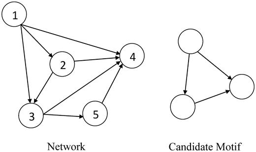
An example directed graph and a candidate motif.
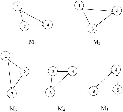
Instances of a candidate motif in the network given in Figure 2 using frequency concept F1.
| Concept | Node overlap | Edge overlap | Frequency | Matches |
|---|---|---|---|---|
| F1 | Yes | Yes | 5 | {M1 , M2, M3, M4, M5} |
| F2 | Yes | No | 2 | Either {M1 , M4} or {M3, M4} |
| F3 | No | No | 1 | One of {M1 , M2, M3, M4, M5} |
| Concept | Node overlap | Edge overlap | Frequency | Matches |
|---|---|---|---|---|
| F1 | Yes | Yes | 5 | {M1 , M2, M3, M4, M5} |
| F2 | Yes | No | 2 | Either {M1 , M4} or {M3, M4} |
| F3 | No | No | 1 | One of {M1 , M2, M3, M4, M5} |
| Concept | Node overlap | Edge overlap | Frequency | Matches |
|---|---|---|---|---|
| F1 | Yes | Yes | 5 | {M1 , M2, M3, M4, M5} |
| F2 | Yes | No | 2 | Either {M1 , M4} or {M3, M4} |
| F3 | No | No | 1 | One of {M1 , M2, M3, M4, M5} |
| Concept | Node overlap | Edge overlap | Frequency | Matches |
|---|---|---|---|---|
| F1 | Yes | Yes | 5 | {M1 , M2, M3, M4, M5} |
| F2 | Yes | No | 2 | Either {M1 , M4} or {M3, M4} |
| F3 | No | No | 1 | One of {M1 , M2, M3, M4, M5} |
Graph isomorphism
Two graphs are ‘isomorphic’ if there exists a one-to-one mapping between their nodes such that each edge in one graph can be mapped to an edge in the other graph [30]. The graph isomorphism problem—checking if two graphs are isomorphic—is one of a very small number of problems belonging to ‘NP’ which are neither known to be ‘NP-Complete’ nor known to be solvable in polynomial time [31]. The best known algorithm has a run-time of  for graphs with n vertices [32, 33]. However, the sub-graph isomorphism problem—checking if a network G contains an isomorph of another graph g—is NP-Complete [34]. Isomorphism can be solved by using ‘Canonical Labeling’ of its nodes [35]. Practical algorithms such as the NAUTY [36] have been used in several motif finding tools for isomorphism testing.
Statistical significance
When frequencies of all size-k sub-graphs are known in both the input and random networks, different thresholds and metrics are applied to determine which sub-graphs are significantly frequent.
Thresholds

 be the mean of frequencies of gk in the random networks. Then, gk is ‘unique’ if
Significance metrics
 and σ2random be the mean and variance of frequencies of gk in a sufficiently large set of random networks, respectively. The z-score is defined as the difference of finput and
  , divided by the standard deviation σ2random. Namely, the z-score is calculated as,
The P-value represents the probability of a motif to appear an equal or greater number of times in a random network than in the given input network. A motif is usually regarded as ‘statistically significant’ if the associated P-value is less than 0.01 or z >2.0.

 frequency of gk in G is significant with 99% confidence. Note, it has been pointed out that many properties of biological networks are non-Gaussian [25, 37], and probability distribution of frandom should be estimated from the input network through various estimation techniques [38].
 is a small positive number preventing the ratio from approaching infinity when the frequencies are small. The value of Δ usually ranges between −1 (under-represented) and 1 (overrepresented). Another metric, the motif ‘significance profile’ (SP), is defined as a vector of z-scores of a particular set of motifs, which is normalized to a length of one [15]. Let n be the number of motifs in the set, and zi be the z-score of the i-th motif. The motif SP of the i-th motif in the set is thus calculated as,
Random graphs

It is essential for the generated random graph to resemble the original graph in terms of global properties such as the average degree, diameter, average path length, degree distribution and frequency of particular topological sub-structures, etc [1]. (Note the terms here follow the definitions in graph theory. For example, the ‘average degree’ is the average number of adjacent edges of the nodes in a graph; the ‘diameter’ of a graph is the maximum of the shortest paths of all vertex pairs, etc.)
The most common random graph generation technique used in motif finding algorithms is the ‘Switching Method’. It repeatedly selects two random edges, a→b and c→d, in the network, and exchanges the ends to form two new edges a→d and b→c. The randomized graph has the same node and edge counts as in the input network, and the in- and out-degrees of the nodes are preserved. The switching method has also been widely applied in studying such features of biological networks as modularity and degree correlation. This method has a drawback that one cannot be certain when the network is adequately randomized. However, numerical studies have shown that, for many networks, 100*E times of switching appear to be adequate to achieve randomization, where E is the number of edges [3].
An alternative algorithm for random graph generation is the ‘Matching Method’, where each vertex is assigned a set of ‘stubs’—the sawn-off ends of incoming and outgoing edges—according to the desired degree sequence. The in-stubs and out-stubs are then picked randomly in pairs and ‘fused’ to create the network edges. Although minor adjustments are needed to tend to real-world networks, where only a rather minority of nodes have a high degree, the matching algorithm usually correctly generates random networks with the desired properties [3].
The network motif-finding problem is thus defined as follows. Given the following inputs:
- G
a network represented as a directed or undirected graph.
- K
the maximum size of motif to search in G.
- P
the required confidence level.
- F
frequency threshold.
- U
uniqueness threshold.
- N
number of random networks.
Find all k-node sub-graphs {gk} with 2 ≤ k ≤ K occurring in G such that the frequency (or other metrics such as the concentration) of gk in G is:
Above the given thresholds (Equations 1 and 2).
Significantly higher than that in the random graphs with confidence level associated with P (Equation 4) in terms of either
z-score (Equation 3), or
Abundance (Equation 5), or
SP (Equation 6).
STRATEGIES FOR MOTIF FINDING ALGORITHMS
In this section, we discuss several solution strategies for different parts of the motif-finding problem. There are three major parts of the problem: performing sub-graph census, solving graph isomorphism and ensuring that one sub-graph gets accounted for exactly once. The ‘pattern growth’ method is widely used in order to systematically explore or generate possible sub-graph variations. Strategies used in sub-graph census include exact ‘enumeration’, ‘sampling’ and ‘mapping’. Some strategies for isomorphism checking include ‘explicit checking’ (using canonical labeling or NAUTY [36]) and ‘symmetry breaking’ coupled with ‘mapping’. We present some representative motif finding algorithms under a simple classification scheme based on the strategies the different algorithms use. These algorithms are MAVisto [28, 42], NeMoFinder [43], Kavosh [20], MFinder [39, 44], FANMOD [40, 45], Grochow and Kellis [21] and MODA [27]. Table 2 illustrates how different strategies can be combined to solve the motif-finding problem. Note that some comparisons made in this and the following sections are partially based on experimental results reported by articles accompanying the algorithms mentioned above. Web-based tools of some algorithms are freely available for scientific use and can be accessed at the following sites:
MFinder: http://www.weizmann.ac.il/mcb/UriAlon/groupNetworkMotifSW.html
FANMOD: http://theinf1.informatik.uni-jena.de/~wernicke/motifs/index.html
MAVisto: http://mavisto.ipk-gatersleben.de/
Summary of strategies adopted by different algorithms
| Network centric | Sampling | Pattern growth | Mapping | Symmetry breaking | Isomorphism checking | |
|---|---|---|---|---|---|---|
| MAVisto | Yes | No | Yes | No | No | Canonical labeling |
| NeMoFinder | Yes | No | Yes | No | No | Canonical labeling |
| Kavosh | Yes | No | Yes | No | No | NAUTY |
| MFinder | Yes | Yes | Yes | No | No | |
| FANMOD | Yes | Yes | Yes | No | No | NAUTY |
| Grochow | No | No | No | Yes | Yes | Sym-break, mapping |
| MODA | No | Yes | Yes | Yes | Yes | Sym-break, mapping |
Pattern growth tree
A systematic way of generating a large set of variants from a base sub-graph is to extend it one step at a time by modifying one of its nodes or edges, and use the extended sub-graph to generate further variants. This sequence of action can be viewed as a tree (much like a search tree), where each node of the tree holds one sub-graph, and its children hold sub-graphs extended from that node so that a graph at a parent node is a sub-graph of all nodes in its sub-tree. This strategy, called ‘pattern growth tree’, can be used to systematically generate all possible size-k graphs starting with a size-k tree (‘Generating all sub-graphs of a given size’ section). It can also be used to systematically enumerate all occurrences of size-k sub-graphs in the target network.
Pattern growth strategy, when coupled with appropriate constraints, yields several benefits. When searching for size-k sub-graphs in the network, a pattern growth tree built for size-(k-1) sub-graphs can be reused. This may lead to significant improvements in computational cost, which is exploited by MODA (‘Motif-centric algorithms’ section). Moreover, through a careful extension process one can guarantee that each sub-graph appears only once in the pattern growth tree, thus saving redundant computation. This is exploited by Kavosh (‘Network-centric algorithms’ section). Also, suppose the sub-graph at any node of the pattern growth tree violates a constraint. For example, its frequency falls below the frequency threshold, or becomes higher than the frequency of its ancestor (thus breaking downward closure property, if applicable). This information can be used to prune sub-trees rooted at that node, leading to increased computational efficiency. This is exploited by MAVisto (‘Network-centric algorithms’ section).
Sub-graph census: exhaustive versus sampling
Sub-graph census is the process of scanning the target network (node-by-node or edge-by-edge) and enumerating all occurrences of all sub-graphs of a given size. Usually this is done using a pattern growth tree. In general, the number of sub-graphs in a network increases exponentially when the network size increases: there are up to  matches for a sub-graph g in the target network G under frequency concept F1, where
  and
and  are edge counts in G and g, respectively [28]. The exhaustive census is therefore a time-consuming process, especially when the network or the sub-graph to be enumerated is large.
One can adopt a probabilistic approach by taking an adequate number of random size-k sub-graph samples from the original network. As is the case with probabilistic algorithms, with a good amount of trials one can expect to get closely accurate yet quick results, but with non-zero probability that some potential motifs will be missed. This is called the ‘sampling strategy’ for sub-graph census. Sampling saves much computation, thus allowing us to discover larger motifs. Moreover, sampling makes the algorithm insensitive to the size of the target network.
For each sub-graph in the pattern growth tree, an ‘edge-sampling’ strategy [39] randomly picks an edge from the network and selects a size-k sub-graph around that edge from the network for comparison. MFinder (‘Algorithms with sampling—MODA’ section) uses this strategy. However, it turns out that this is ‘biased sampling’: the probability of picking all size-k sub-graphs is not uniform in this strategy because sub-graphs having more edge are likely to be counted more, forcing the algorithm to assign specific weight to each sub-graph (and remember the sub-graph and the weight) to balance off the recounting, which leads to excessive memory usage. Edge extension in the pattern growth tree also encounters the same sub-graphs multiple times, causing redundant computation.
The ‘node-sampling’ strategy [40, 45], however, is able to ensure uniform probability of picking any size-k sub-graphs. It assigns to each level of its pattern growth tree a probability that the nodes (of the pattern growth tree) at that level will be further explored. It then probabilistically traverses the pattern growth tree, which guarantees that all the terminal nodes (size-k graphs) will be explored with equal probability, thus eliminating the memory drawback of edge-sampling strategy. Also, careful node extension in the pattern growth tree can ensure that a particular sub-graph will be encountered exactly once, which avoids redundant computation. FANMOD (‘Network-centric algorithms’ section) uses this strategy, as it is significantly efficient and faster than edge-sampling.
In some networks (termed scale-free) the sub-graph aggregation around high-degree nodes is higher than around low-degree nodes [46]. While not all biological networks are scale-free, this case was verified in empirical studies [27]. Thus, there is a variant of node-sampling strategy which probabilistically picks a node depending on its degree. MODA (‘Motif-centric algorithms’ section) uses this strategy.
Generating all sub-graphs of a given size
Algorithms for computing frequency of any ‘given’ sub-graph over the target network (as opposed to sub-graph census, which computes frequency of all sub-graphs of a given size) must generate all possible non-isomorphic variants of that sub-graph. This can be done using a pattern growth tree, as in MODA [27], or by generating all isomorphic classes of a sub-graph using external tools [46], as in Grochow and Kellis [21]. This strategy has the drawback that when the size of the sub-graph gets >10, computations due to the number of possible variants become intractable [23, 47–49]. Another disadvantage is that this process generates and computes frequency for sub-graphs that might not occur in the target graph. One should note that isomorphism is partly resolved even before enumerating sub-graphs in the target network.
Mapping
The mapping strategy [21] of finding sub-graph instances takes a size-k sub-graph (candidate motif) and maps it onto the network in as many different places as it can. This is the opposite view of enumerating all size-k sub-graphs in the network and then computing frequency of a candidate size-k motif. A mapping strategy ranks the nodes in the target network based on their (and their neighbors’) degree properties, and then looks for nodes in the input network that have similar characteristics of nodes in the candidate motif [21, 50]. This strategy is introduced by Grochow and Kellis [21] and is also used by MODA (‘Motif-centric algorithms’ section). Mapping, when used with symmetry breaking (‘Symmetry breaking’ section), resolves isomorphism without explicit checking [21].
Symmetry breaking
The symmetries of a graph are known as ‘automorphisms’, or self-isomorphisms. The group of automorphisms are in the same ‘equivalence class’. One can specify a set of symmetry breaking conditions [21] for each equivalence class. Checking if these conditions hold between two graphs is easier than checking the isomorphism. Algorithms that use symmetry breaking while generating candidate motifs can prevent many isomorphism computations, thus increasing efficiency. This strategy is used alongside mapping. It was introduced by Grochow and Kellis,and was also used by MODA (‘Motif-centric algorithms’ section).
Motif finding algorithms
We discuss a simple framework for describing a network motif finding algorithm based on the strategies it uses. Under this framework, we discuss some representative algorithms (Table 3). Note these algorithms are selected not by their performance, but by the particular strategies they use. These algorithms are classified into two broad classes—‘network-centric’ and ‘motif-centric’ algorithms—which can be further classified depending on whether a sampling strategy is used while counting sub-graph frequencies.
Network-centric algorithms
Network-centric algorithms start with the network. They enumerate all sub-graphs with size k that occur in the target network. Network-centric algorithms have the benefit that sub-graphs that do not occur in the target network are never encountered. However, these algorithms cannot compute the frequency of a given sub-graph without doing sub-graph census.
Algorithms with exact census—MAVisto, NeMoFinder and Kavosh
MAVisto stands for ‘Motif Analysis and Visualization Tool’. Developed by Schreiber and Schwöbbermeyer [42] in 2005, MAVisto is a network-centric algorithm that uses a pattern growth method called FPF (Flexible Pattern Finder) [28]. It uses the downward closure property commonly used in data mining, as well as a frequency threshold to prune branches of the pattern growth tree.
The ‘Network Motif Finder’, NeMoFinder, was developed in 2006 by Chen et al. [43]. Dedicated to undirected, unlabeled PPI networks, the NeMoFinder finds motifs that are maximal [51] (i.e. not contained in any other motif), are unique sub-graphs, but not necessarily induced. (Note H is an ‘induced’ sub-graph of G if it has exactly the edges that appear in G over the same vertex set.) It uses frequency and uniqueness thresholds, and the F1 frequency concept. Notably, the input network is partitioned into smaller sub-networks for enumeration of lower-level sub-graphs in the pattern growth tree, which makes it less-sensitive to large networks. The ‘Canonical Adjacency Matrix’ is used to resolve isomorphism through a method called ‘Graph Cousins’ [27]. This method, however, is likely to produce some redundant isomorphic candidate motifs [27].
Kashani et al. [20] developed Kavosh in 2009. It’s a network-centric algorithm using the pattern growth tree (with node-extension) to enumerate all size-k sub-graphs in the input network. Kavosh adopts the ‘Revolving Door algorithm’ [52] for traversing the pattern growth tree, ensuring that every candidate motif is encountered exactly once. The frequency concept F1 is used, along with a frequency threshold. In addition, Kavosh uses the NAUTY algorithm [36] (‘Graph isomorphism’ section) for isomorphism testing, which is efficient as the NAUTY does not generate any redundant candidate motif [36].
Algorithms using sampling—Mfinder and Fanmod
MFinder was developed in 2005 by Kashtan et al. [44], which showcases their edge-sampling algorithm [39]. The pattern growth tree is used to enumerate all sub-graphs in the network through edge extension. Frequency concept F1 is used, but motifs are required to be induced sub-graphs. MFinder also uses concentration as the significance metric. MFinder is seriously handicapped with drawbacks of edge-sampling, and is not suitable for finding large motifs [26]. MFinder can also perform exhaustive sub-graph census instead of sampling, as an option. In this regard, the MFinder functions as the enumeration algorithm [1].
FANMOD was developed in 2006 by Wernicke et al. [40, 45], which uses a node-sampling strategy and a pattern growth tree using node-extension. FANMOD is fast, and can detect up to size-8 motifs in both directed/undirected networks. It uses F1 frequency concept, and motifs are required to be induced. FANMOD uses concentration as the significance metric and NAUTY [36] for isomorphism checking. FANMOD’s randomized enumeration algorithm is known as Rand-ESU. FANMOD, like MFinder, is also able to do exhaustive census over the target network.
Motif-centric algorithms
Motif-centric algorithms are able to compute frequency of any given sub-graph in the target network. This enables them to directly verify whether the query sub-graph is a motif. In order to compute frequencies of all size-k graphs, a motif-centric algorithm first enumerates all possible size-k graphs. As network-centric algorithms, motif-centric algorithms can be further classified depending on whether sampling is used over the target network while counting sub-graph frequencies.
Algorithms with exact search—Grochow
Devised by Grochow and Kellis [21] in 2007, this algorithm is the first example of a motif-centric algorithm. Grochow uses symmetry breaking with mapping to count the frequency of a query sub-graph. It uses the ‘geng’ and ‘directg’ packages by McKay [53–55] to exhaustively generate all non-isomorphic sub-graphs of size-k; it then checks if any of them is a motif. Grochow is able to exhaustively find seven-node motifs in the Saccharomyces cerevisiae PPI network efficiently. Although mapping is an exact strategy, it is possible to first use sampling to pick a random (potentially large) sub-graph from the network, and then use symmetry breaking and mapping to determine its frequency.
Algorithms with sampling—MODA
MODA, was developed by Omidi et al. [27] in 2009. This motif centric algorithm uses a pattern growth tree, called ‘expansion tree’, which uses symmetry breaking to generate unique extensions. It then uses mapping for the first level of the expansion tree. Information from the previous level is then used to efficiently enumerate the extensions for each subsequent level. Note that MODA implements an improved node-sampling strategy in every level—even for mapping, as opposed to Grochow. Moreover, the expansion tree enables it to reuse computations done for smaller-size query motifs, resulting in its high efficiency. Largely due to this combination of efficient strategies, MODA is fast and can handle rather large networks and motifs. It also allows arbitrary overlap between sub-graphs, using frequency concept F1.
PERFORMANCE COMPARISONS
Selected results from various comparative studies of motif finding algorithms are presented in Tables 4, 6 and Figures 4–7
![Execution times (in seconds) of NeMoFinder, FPF algorithm (MAVisto), MFinder (sampling) and full enumeration algorithm for sub-graphs of sizes 3–13 in a PPI network of S. cerevisiae [54] with 1004 nodes and 957 edges, as reported by Chen et al. [43].](https://oup.silverchair-cdn.com/oup/backfile/Content_public/Journal/bib/13/2/10.1093/bib/bbr033/2/m_bbr033f4.jpeg?Expires=1749311061&Signature=PuR9YHv9n3XNbOneTOSU3XZ3HL5n279iHohCwffN5jPBxGzMD0bKX20vBjr1jyKePNlY0nQViHXqufYaSj4PQHlRYio6ZkF9AyPNqIEBmDSaAJuSNpXPSnu7TezXl5Owstdv2zziAUF1~7RZ6~lfrYGu6F1IZvfARrbd7AanaonZObS5W-PiG3oJOw9ecePerhjoWeXnDHle83sHOdPTtDiP9u1nkZP9yw2cIxDEvbKdSO6T4zXpoJIVCq6226kPDA8tvTzlsEfHHS8tLZr9ySbAPfilnmXkoIwTbK2f41itUL6BhqiIP0HdtXkH27EUOkHFNlsCuh9XRtkj2jINsA__&Key-Pair-Id=APKAIE5G5CRDK6RD3PGA)
![Execution times (in seconds) of MODA, MFinder, Grochow, FPF algorithm and FANMOD for sub-graphs of sizes 3–9 in an E. coli transcription network used by Shen-Orr et al. [2], which is a directed graph of 116 nodes and 477 edges (Courtesy of Omidi et al. [27]). Algorithms were executed on the input network only.](https://oup.silverchair-cdn.com/oup/backfile/Content_public/Journal/bib/13/2/10.1093/bib/bbr033/2/m_bbr033f5.jpeg?Expires=1749311061&Signature=BbUkv5DVvg6f42fACZ76GjwjPOc6yzjjK4ZtVl~HHcJdH7IQ443SJK0VTZMO98gscWE-htSyPoJ-q9oWHAC5B~vZ6kezu~6nGoCA-jiD-ZbXDKbkpKr49uBDtzdJctpoJ9etRWbccg~xJ8W7N~m32208vrJEv0HCZITo2amX8beQFnwjaIR0G8R3m2aRw2lq9AB0atSxPaBjvxROSnyF4tJQBxo9JWUBSeXBjywNPtWJoW3DC8AMQaS0acUSPdK07EVXG0TvBPydSpEvw3AkkOXFaB9SE8ROhZxNxd5vk7sAl02jEm4c2RnKhKs6QlzwKb8lEQKqQsbSG4ZeNRRLXA__&Key-Pair-Id=APKAIE5G5CRDK6RD3PGA)
Execution times (in seconds) of MODA, MFinder, Grochow, FPF algorithm and FANMOD for sub-graphs of sizes 3–9 in an E. coli transcription network used by Shen-Orr et al. [2], which is a directed graph of 116 nodes and 477 edges (Courtesy of Omidi et al. [27]). Algorithms were executed on the input network only.
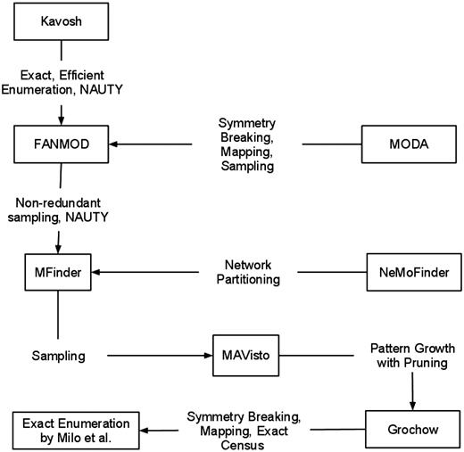
How the combination of strategies affects performance of an algorithm. An arrow from algorithm A to algorithm B implies that A usually outperforms B for larger networks and motifs. Each arrow is labeled with the strategies used in A that contribute to the dominance.

Execution times (in seconds) of Kavosh, FANMOD, MAVisto and MFinder for sub-graphs of size 3–10 in various networks
| Network | k | Kavosh | FANMOD | MAVisto | MFinder (exhaustive) |
|---|---|---|---|---|---|
| E. coli | 3 | 1 | 1 | 14,000 | 30 |
| 4 | 2 | 3 | 300 | ||
| 5 | 15 | 16 | 23,000 | ||
| 6 | 140 | 130 | |||
| 7 | 1400 | 1200 | |||
| 8 | 13,000 | 9000 | |||
| 9 | 100,000 | ||||
| 10 | 1,000,000 | ||||
| Social | 3 | 1 | 1 | 400 | 10 |
| 4 | 1 | 1 | 1500 | 50 | |
| 5 | 2 | 3 | 800 | ||
| 6 | 10 | 20 | 180,000 | ||
| 7 | 70 | 100 | |||
| 8 | 400 | 800 | |||
| 9 | 2600 | ||||
| 10 | 15,000 | ||||
| S. cerevisiae | 3 | 2 | 3 | 16,000 | 30 |
| 4 | 30 | 40 | 300 | ||
| 5 | 1000 | 1100 | 34,000 | ||
| 6 | 20,000 | 24,000 | |||
| 7 | 750,000 | 900,000 | |||
| 8 | 17,000,000 | 19,000,000 | |||
| 9 | 300,000,000 | ||||
| 10 | 7,000,000,000 |
Note: Here k denotes a sub-graph size. Note that large numeric values have been rounded to improve visualization (Courtesy of Kashani et al. [20]).
Input networks used in the comparisons made in Table 6
| Network | Nodes | Edges | Description |
|---|---|---|---|
| Circuit | 252 | 399 | Electronic circuit |
| Yeast | 688 | 1079 | S. cerevisiae transcriptional network |
| Social | 1000 | 15541 | Social network with heterogeneous communities |
| Network | Nodes | Edges | Description |
|---|---|---|---|
| Circuit | 252 | 399 | Electronic circuit |
| Yeast | 688 | 1079 | S. cerevisiae transcriptional network |
| Social | 1000 | 15541 | Social network with heterogeneous communities |
Execution times (in seconds) of MFinder, FANMOD and Grochow, all with exhaustive census on the input networks
| Network | k | MFinder | FANMOD | Grochow |
|---|---|---|---|---|
| Circuit | 4 | 0.10 | 0.05 | 0.36 |
| 5 | 0.36 | 0.14 | 15.79 | |
| 6 | 2.45 | 0.67 | 2519.3 | |
| 7 | 17.54 | 4.34 | >4h | |
| 8 | 130.66 | 27.46 | >4h | |
| 9 | MEM | 140.66 | >4h | |
| Yeast | 4 | 2.42 | 0.77 | 2.25 |
| 5 | 55.67 | 15.21 | 107.82 | |
| 6 | MEM | 260.38 | >4h | |
| 7 | MEM | 5023.91 | >4h | |
| Social | 4 | 40.44 | 11.22 | 16.98 |
| 5 | MEM | 281.40 | 1122.74 | |
| 6 | MEM | 7951.47 | >4h |
Note: Here k indicates the motif size. MEM indicates the out-of-memory situation (Courtesy of Ribeiro et al. [26]).
Sampling strategies for sub-graph census are faster
FANMOD is efficient in computation and tends to produce results while other exact algorithms (except Kavosh) struggle (Figure 5, Tables 4 and 6). Exact sub-graph census becomes slow as either network or motif size increases, as demonstrated in MAVisto on various occasions (Figures 4 and 5, Table 4). However, NeMoFinder, which is a network-centric tool doing exact census, shows promise in finding large motifs in large PPI networks (Figure 4) as the algorithm works by partitioning the input network and thus effectively reducing the problem size. Similarly, Kavosh, yet another network-centric algorithm with exact census, is sometimes faster than FANMOD and can find larger motifs than FANMOD (Table 4), largely due to the highly efficient sub-graph enumeration strategy of Kavosh and its use of NAUTY [36] for isomorphism checking (‘Network-centric algorithms’ section). Both MODA and FANMOD use the sampling strategy for sub-graph census. FANMOD is faster than MODA (Figure 5) since MODA, a motif-centric tool, considers more sub-graphs than FANMOD. However, MODA can find larger motifs than FANMOD (Figure 5), partly because of a more efficient isomorphism-checking strategy by mapping and symmetry breaking, and partly because of its ability to reuse results from earlier computations (‘Motif-centric algorithms’ section).
Motif-centric algorithms tend to slow down as sub-graph size grows
The effect is observable in all algorithms, but more so in motif-centric algorithms such as the Grochow (Table 6 and Figure 5). Grochow is more efficient than the exact enumeration algorithm [1] due to its symmetry breaking techniques that enables it to reduce redundant counts of sub-graphs. Yet Grochow is found to be slower than MAVisto (Figure 5) and the exhaustive version of MFinder (Table 6), highlighting the limitation of generating all possible size-k sub-graphs. However, as mentioned previously, MODA could detect larger motifs than does FANMOD, although FANMOD is faster (Figure 5). Nevertheless, motif size is a bottleneck for motif-centric tools.
MAVisto and MFinder are limited in motif size
The MFinder stores all sub-graphs in memory and considers the same sub-graph many times. Thus MFinder scales poorly with motif size despite its use of sampling for sub-graph census. Table 6 shows that MFinder (exact census) takes more memory and time than FANMOD (exact census), since FANMOD counts a sub-graph only once. Similar observations can be made in Figure 5 and Table 4. MAVisto, on the other hand, performs poorly (Figures 4, 5 and Table 4) mainly because it does exact census in a less sophisticated way than Kavosh does.
Which tool should one use for larger motifs?
Although current motif finding algorithms are able to find only small motifs when the target network is large and/or dense, one may argue that if an exact result is necessary, Kavosh will be a desirable tool. Otherwise, FANMOD or MODA will be a good choice. In addition, NeMoFinder is a good choice for large PPI networks.
What are the bottlenecks for performance?
The most obvious bottleneck is the number of random graphs used for comparison. While computing over a large number of random graphs will statistically justify the overrepresentation of motifs, it is clearly a time-consuming process. The second bottleneck is the target network size. Real-world networks tend to be large, and doing exact sub-graph census is not always practical. The third bottleneck is the sub-graph size. When looking for motifs with more than 8–10 nodes, the number of possible sub-graphs becomes prohibitively large (depending on the available computational resources). It affects motif-centric algorithms in particular, and all algorithms in general when the target network is large and dense.
Figure 6 illustrates which strategy makes an algorithm better than others. In this figure, rectangles denote algorithms and arrows denote the dominance between two algorithms. Each arrow is labeled with the strategies that result in the superior performance. We placed MODA over FANMOD in Figure 6 since MODA can find larger motifs as shown in Figure 5, although their execution times are comparable. From this figure one can get a quick understanding of how strategies discussed in ‘Strategies for motif finding algorithms’ section affect the performance of algorithms. There are no arrows among Kavosh, MODA, and NeMoFinder as they have not been comparatively studied in the literature.
CONCLUSIONS AND FUTURE DIRECTIONS
Solving the network motif-finding problem involves several aspects in research—generating random graphs, checking graph isomorphism, estimating sub-graph frequencies in the network (by exact enumeration or sampling) and generating the set of candidate motifs, etc. Each has challenges and possibilities of its own. While several algorithms exist in the literature with experimental results available on selected target networks, the relative performance when varying other topological features of the networks such as clustering coefficient, scale-freeness, etc need to be further studied to conclude their strengths, weaknesses and the practical relevance.
One research direction toward improving these algorithms is to devise a robust, parallel algorithm for a distributed computation platform that could simultaneously analyze different parts of the network, thus reducing the execution time and enabling our reach to larger motifs and networks.
While checking isomorphism for general graphs involves work in exponential time, polynomial-time algorithms do exist for special graphs such as the planar graphs, interval graphs, and the two-connected series-parallel graphs, etc [55]. If some biologically verified (large) motifs have similar topological characteristics that enable a fast isomorphism test, one could prioritize expected outputs of a motif finding algorithm to generate those with such topologies first. This will allow us to generate highly relevant (large) motifs early, if they exist, during the computation process.
Another improvement could be made by reducing unnecessary computations over the random graphs. After performing sub-graph census over the input network, the set of possible motifs is already limited to the sub-graphs found in the census. The same computation over hundreds (or thousands) of random networks is then performed to compute frequencies for sub-graphs, many of which may not occur in the target networks. Such computations can be saved by a more efficient data structure to keep track of candidate motifs.
Network motif finding algorithms can be divided into network-centric and motif-centric groups.
Network motif finding algorithms can be further classified based on their use of probabilistic sampling of the target network.
Efficient combination of different strategies leads to a better performance.
FUNDING
This work was supported by the National Science Foundation [CCF-0755373 to E.W., B.B., S. Q. and C.-H.H.]; and the National Institutes of Health [R13-LM008619 to C.-H.H.].
