


Abstract
Dormancy of buds is an important phase in the life cycle of perennial plants growing in environments where unsuitable growth conditions occur seasonally. In regions where low temperature defines these unsuitable conditions, the attainment of cold hardiness is also required for survival. The end of the dormant period culminates in budbreak and flower emergence, or spring phenology, one of the most appreciated and studied phenological events – a time also understood to be most sensitive to low-temperature damage. Despite this, we have a limited physiological and molecular understanding of dormancy, which has negatively affected our ability to model budbreak. This is also true for cold hardiness.
Here we highlight the importance of including cold hardiness in dormancy studies that typically only characterize time to budbreak. We show how different temperature treatments may lead to increases in cold hardiness, and by doing so also (potentially inadvertently) increase time to budbreak.
We present a theory that describes evaluation of cold hardiness as being key to clarifying physiological changes throughout the dormant period, delineating dormancy statuses, and improving both chill and phenology models. Erroneous interpretations of budbreak datasets are possible by not phenotyping cold hardiness. Changes in cold hardiness were very probably present in previous experiments that studied dormancy, especially when those included below-freezing temperature treatments. Separating the effects between chilling accumulation and cold acclimation in future studies will be essential for increasing our understanding of dormancy and spring phenology in plants.
INTRODUCTION
Dormancy, along with development of cold hardiness in tissues, allows plants to survive unsuitable growing conditions during winter and precisely time their budbreak upon return of suitable temperatures in spring. Cold hardiness refers to the minimum temperature which plants can viably withstand – a dynamic trait that is generally elicited by low-temperature exposure. Chilling accumulation – a thermal time accrued through exposure to moderately low temperatures (~0–10 °C) – promotes the transition from the initial warm temperature non-responsive phase of dormancy to the warm temperature-responsive phase due to ontogenetic changes within buds [often referred to as the endo- to ecodormancy transition – see Lang et al. (1987) for definitions]. This change in temperature responsiveness is observed in experiments as decreased time to budbreak upon transfer to forcing conditions – the exposure to warm temperatures and long daylength. The molecular and physiological basis for dormancy and its transitions, including the precise range of temperatures eliciting chill accumulation responses, remain only partially understood (Cooke et al., 2012; Yamane et al., 2021). As a result, particularly due to the lack of knowledge on which and how temperatures promote chilling, modelling chilling accumulation across different regions (Luedeling and Brown, 2011) and modelling time to budbreak in spring (spring phenology) (Melaas et al., 2016; Wang et al., 2020; Zohner et al., 2020) present a linked challenge.
Here we show that the phenotype of time to budbreak, which has been used in the vast majority of experiments for over a century, only tells part of the story. This may have limited greater advances in our understanding of dormancy from a mechanistic standpoint (including the qualitative interpretation of dormancy), and related aspects such as the development of accurate chilling accumulation and spring phenology models, which is an important component of Earth system models (Richardson et al., 2012; Chen et al., 2016). We propose that evaluation of cold hardiness and cold deacclimation (the decrease in cold hardiness over time due to warm temperature exposure, hereafter referred to as only deacclimation) can enhance interpretations that to date have been based solely on time to budbreak to phenotype dormancy completion as influenced by chilling accumulation. To support our perspective, we present a combination of small original datasets, as well as apply and discuss our proposed interpretation to some cases within the literature.
BUDBREAK, THE MAIN DORMANCY PHENOTYPE
The first presumed report of low-temperature exposure (chilling) as a requirement for proper budbreak of temperate species upon warm temperature exposure (forcing) is over two centuries old (Knight, 1801). Chilling–forcing experiments went on to become the standard approach to study dormancy for the past 100 years (Coville, 1920). In these experiments, plants [or cuttings as valid proxies for whole plant responses (Vitasse and Basler, 2014)] are subjected to low temperatures for varying durations (chilling treatments), either naturally (field) or artificially (low-temperature chambers), and then transferred to forcing conditions to monitor regrowth. Chill accumulation is thus a thermal time related to the interaction between temperature during chill treatment (thermal) and duration of chill treatment (time) that plants are exposed to. The typical metrics recorded in chilling–forcing assays are based on visual observation of percentage budbreak (Alvarez et al., 2018; Shellie et al., 2018; Baumgarten et al., 2021) and/or time to budbreak (Londo and Johnson, 2014; Alvarez et al., 2018; Shellie et al., 2018; Baumgarten et al., 2021; Kovaleski, 2022) upon exposure to forcing conditions. A longer duration of chilling treatments correlates with higher percentage budbreak and shorter time to budbreak (i.e. negative correlation between chilling accumulation and heat requirement under forcing). We posit, however, that in most studies the temperature treatments applied as chilling are also inadvertently affecting other physiological aspects in the buds beyond dormancy progression, in particular cold hardiness.
While artificial chilling treatments are often described as constant, positive temperatures [e.g. 1.5 and 4 °C in Flynn and Wolkovich (2018)], more and more studies have included negative temperatures to study their effect on chilling accumulation [–3, –5 and –8 °C in Cragin et al. (2017); –2 °C in Baumgarten et al. (2021)]. However, these experiments have not included evaluations of cold hardiness in response to chilling. The combined effects of chilling and cold hardiness on time to budbreak have only been studied in field conditions, although this has now been done in many species, both of fruit crops, such as grapevines (Kovaleski et al., 2018; Kovaleski, 2022; North et al., 2022) and apricot (Kovaleski, 2022), and other ornamental and forest species (Lenz et al., 2013; Vitra et al., 2017; Kovaleski, 2022). However, artificial chilling experiments are key to better understand the effects of particular temperatures in providing chilling, as field conditions are too variable for this.
COLD HARDINESS INFLUENCES TIME TO BUDBREAK
Using grapevine cuttings of five different cultivars (all Vitis interspecific hybrids), we supplied chilling using three treatments: constant (5 °C), fluctuating (daily fluctuations of –3.5 °C for 7 h, followed by 6.5 °C for 17 h), and field-collected cuttings in Madison, WI, USA. When evaluating cold hardiness of buds, we observed that the fluctuating treatment elicited a greater gain in cold hardiness over time compared to constant conditions, while both were surpassed by buds subjected to much lower temperatures in the field (Fig. 1A). After 2.5 months under treatments, some cuttings from the constant and fluctuating treatments were reciprocally exchanged. Cold hardiness was again evaluated 1 month after the reciprocal exchange: field buds were still the most cold hardy, followed by all treatments which had been at any point exposed to fluctuating conditions, while buds that remained in the constant temperature treatment were the least cold hardy (Fig. 1B, bottom). Cuttings from the same treatments, when placed under forcing conditions (22 °C, 16 h/8 h day/night) for evaluation of time to budbreak at the end of the experiment, demonstrated a similar, but opposite distribution: field-collected cuttings took the longest to break bud, whereas constant temperature-treated buds took the least amount of time (Fig. 1B, top). All treatments reduced time to budbreak compared to the first collection in mid-October when average time to budbreak was >120 days. Based on the observations of time to budbreak alone, the interpretation would be that the constant temperature treatment was the most effective in supplying chilling to buds, leading to shorter time to budbreak compared to fluctuating and field conditons. However, even though exposure to all treatments reduced the time to budbreak by providing considerable chilling, the chilling effects in fluctuating and field treatments would be inadvertently perceived as lower than under constant treatment due to the elongation of time to budbreak attributable to pronounced gains in cold hardiness.
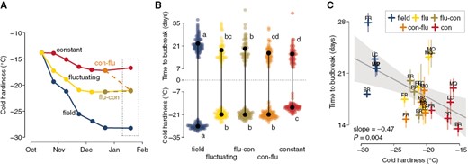
Cold hardiness and time to budbreak relations of grapevine buds in response to different chilling treatments. Cuttings of five Vitis interspecific hybrid cultivars (‘Brianna’ – BR, ‘Frontenac’ – FR, ‘La Crescent’ – LC, ‘Marquette’ – MQ, ‘Petite Pearl’ – PP) were exposed to three different chilling treatments: constant temperature (5 °C), fluctuating temperature (–3.5 and 6.5 °C, for 7 h, 17-h intervals daily), and field temperatures (in autumn and winter of 2020–2021, Madison, WI, USA). After 2.5 months under treatment, cuttings from the artificial chilling treatments were reciprocally exchanged for 1 month of additional chilling (i.e. flu-con and con-flu). (A) Cold hardiness of all original treatments was measured using 15 buds at bi-weekly intervals until the exchange point, and a final cold hardiness measurement was performed 1 month after the exchange. (B) Pairwise comparisons of cold hardiness and time to budbreak under forcing conditions (22 °C, 16-h/8-h day/night) for all cultivars combined using Fisher’s LSD test at α = 0.05. (C) Linear model showing the relationship between time to budbreak and cold hardiness of individual cultivar samples. Standard error of observations is illustrated as semi-transparent extensions from points horizontally (time to budbreak) and vertically (cold hardiness).
The relationship between time to budbreak and cold hardiness provides us with additional information. A slope of about –0.5 d C−1 is observed when looking at the relationship of cold hardiness to time to budbreak (Fig. 1C). This means that for every additional 2 °C of cold hardiness, buds will take an additional day to break bud. The inverse of this slope is also useful: if we consider budbreak occurs at the end of the cold hardiness loss period, we can estimate a deacclimation rate of ~2 °C d−1 based on these data [which is comparable to the maximum deacclimation rate reported by North et al. (2022) for the same cultivars].
This effect is not confined to Vitis spp.: buds of many other species, both angiosperms and gymnosperms, deciduous and evergreen, gain cold hardiness during exposure to low temperatures, particularly when negative temperatures are included in treatments [Fig. 2A; see also hardening treatment in Vitra et al. (2017)]. The relevance of gains in cold hardiness in relation to time to budbreak depends on how much each species responds (Fig. 2B) (where higher gains will have a greater effect) and how quickly any given species loses cold hardiness (see Box 1).
Buds are cold hardy to varying degrees in winter, but most cold hardiness is lost upon budbreak (Lenz et al., 2013; Vitra et al., 2017; Kovaleski et al., 2018; Kovaleski, 2022). The amount of cold hardiness and how it is lost can affect the timing of budbreak. The conceptual examples here are based on extensive phenotyping of 19 species in ten families (within both angiosperms and gymnosperms) that use supercooling as a mechanism of cold hardiness [over 1000 total assays combining both deacclimation and budbreak within published datasets (Kovaleski et al., 2018; Kovaleski, 2022; North et al., 2022)]. Supercooling is a process through which water can remain in a liquid state below its equilibrium freezing point. We expect a similar dynamic for plants that use other mechanisms such as ice tolerance [see Neuner et al. (2019) for extensive description of each mechanism and species within each group] given the similarity in curve shapes of chilling–forcing assays (see fig. 4 in Cannell and Smith, 1983). For species that do not supercool, different types of (generally more labour-intensive) cold hardiness phenotyping is required, such as electrolyte leakage, visual damage or magnetic resonance imaging (Neuner et al., 2019; Kovaleski & Grossman, 2021; Villouta et al., 2021, 2022). Under forcing (i.e. exposure to warm temperatures and generally long days), cold hardiness is lost linearly, without changes in external morphology (Box 1A) [but internal anatomical and morphological changes occur (Viherä-Aarnio et al., 2014; Xie et al., 2018; Kovaleski et al., 2019; Villouta et al., 2022)]. As growth resumes, the supercooling ability has been lost and concentration mostly drives the cold hardiness of tissues. The minimum cold hardiness is thus observed at budbreak and early leafout (Chamberlain et al., 2019), when influx of water driving turgor of tissues leading to budbreak prior to influx of carbohydrates decreases the cellular concentration in bud tissues to a minimum. The relative alignment of these factors may vary based on a given definition of budbreak and/or morphological differences across species (Lancashire et al., 1991; Finn et al., 2007).
Cold hardiness is lost linearly relative to time under forcing conditions at a given temperature for many species (Kovaleski et al., 2018; Kovaleski, 2022; North et al., 2022). Here, this is illustrated conceptually using an orthogonal triangle. The time to budbreak is the base of the triangle, and cold hardiness is the height of the triangle. The deacclimation rate (rate of cold hardiness loss) thus becomes the angle of the hypotenuse to the base of the triangle. Mathematically, these relations are represented by the following equation (from Kovaleski, 2022):
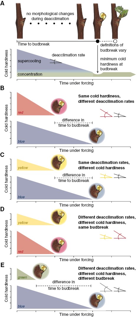
BoxFig 1. The time to budbreak is affected by degree of cold hardiness and deacclimation rate, as budbreak occurs once supercooling ability is lost. (A) In many species, cold hardiness of buds is determined by supercooling ability and cellular concentration. Upon budbreak, supercooling ability has been lost, and cold hardiness is minimal as cellular concentration drops due to high turgor of tissues, with some being recovered as tissues mature. (B–E) Different scenarios are presented where: initial cold hardiness is the same for blue and red triangles (4 arbitrary units), but lower for green and yellow triangles (2 arbitrary units); deacclimation rates are the same for blue and yellow triangles, but greater for red and green triangles; and in combination resulting in time to budbreak being the shortest for green triangle (1 time unit), the same for yellow and red triangles (2 time units), and longest for the blue triangle (4 time units).
where CH0 is the initial cold hardiness, CHBB is the cold hardiness at budbreak, Ψdeacc is the deacclimation potential at the time the forcing assay begins (a rate-limiting proportion that is a function of chill accumulation, thus representing dormancy progression responses), and max is the maximum deacclimation rate at a given forcing temperature (a function of temperature and species/genotype). Three scenarios are explored here where variations in cold hardiness and deacclimation rate affect the timing of budbreak.
In the first example (Box 1B), buds have the same initial cold hardiness, but deacclimate at different rates (red has a higher rate than blue), thus leading to different times to budbreak (earlier for red than for blue). This may be caused by two different factors. One is the different levels of chill accumulation within the same species (or same genotype within a species), where one has higher deacclimation potential, which indicates buds are at different dormancy states. The second factor would be if different species/genotypes are evaluated at the same chill accumulation where one has an inherently faster deacclimation rate. Although both cases increase the denominator within eqn (1), thus decreasing time to budbreak, the source of the effect is different.
In the second example (Box 1C), buds have different initial cold hardiness (blue is more cold hardy than yellow), but deacclimate at the same rate. This could happen if buds are collected from the same genotype, at the same chill accumulation, but some buds were exposed to lower temperatures, leading to greater cold acclimation (i.e. buds exposed to temperatures below that of the chilling range gaining more cold hardiness, changing only the numerator of eqn 1). A scenario where this could occur is buds collected in different locations, where one location has lower minimum temperatures than the other. These being the same genotype, having the same deacclimation rate means the buds are at the same dormancy state, regardless of the difference in time to budbreak. We expect this could be the case for grapevine buds in Fig. 1, considering the long duration (3.5 months) of chilling treatments. That is, differences in time to budbreak are mainly due to differences in cold hardiness at the beginning of the forcing assay.
In the third example (Box 1D), both initial cold hardiness and deacclimation rate are different (red is more cold hardy and has a higher rate of deacclimation compared to yellow). Despite these differences, budbreak occurs at the same time as changes in the numerator are compensated for by changes in the denominator. For the same genotype [and thus the same maximum deacclimation rate at a given temperature (constant max )], this could be observed with less cold hardy buds in autumn, breaking bud in the same amount of time as buds collected in mid-winter which are more cold hardy. The increased chill accumulation between the two times leads to increased deacclimation potential (greater Ψdeacc), thus ultimately losing cold hardiness faster (the effective deacclimation rate is the product of max and Ψdeacc). Although budbreak is happening at the same time, the buds are probably at different dormancy states.
In the fourth example (Box 1E), initial cold hardiness and deacclimation rates differ (blue is more cold hardy and has a lower deacclimation rate compared to green). These combined lead to different timings of budbreak. This scenario reflects the most common case when comparing across species, which inherently have different deacclimation rates. However, this can also be found within the same genotype depending on environmental conditions experienced: green has experienced greater chill accumulation than blue (greater Ψdeacc), thus deacclimating faster; however, higher winter temperatures lead to reduced gains in cold hardiness for green as compared to blue.
These scenarios highlight the importance of a dormancy phenotype that integrates cold hardiness and deacclimation. Budbreak phenotyping alone overlooks important physiological differences associated with dormancy. In some cases, an integrated phenotype will support the interpretation of differing dormancy status based on budbreak but will enhance the extent of differences. In other cases, an integrated phenotype could greatly contradict interpretations of dormancy status based on budbreak.
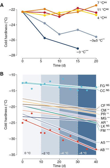
Cold hardiness changes in response to different temperature treatments for different ornamental and forest species. Changes in cold hardiness were analysed using linear models in response to time. (A) Combined effect of temperature treatments on bud cold hardiness of Acer platanoides, A. rubrum, A. saccharum, Cornus mas, Forsythia ‘Meadowlark’, Larix kaempferi, Metasequoia glyptostroboides, Picea abies and Prunus armeniaca. Temperature treatments were constant (–3, 4, 7 and 11 °C) and fluctuating (–8, –3, 2 and –3 °C for 6-h intervals each: ‘−3 ± 5 °C’). (B) Cuttings of 11 species were exposed to decreasing temperatures in –2 °C steps every 10 d from 0 to –6 °C. Linear responses are shown for all species, along with data points for two species: Cercis canadensis (CC) and Abies balsamea (AB). Other species include: FG – Fagus grandifolia; CF – Cornus florida; CM – Cornus mas; PR – Prunus armeniaca; MG – Metasequoia glyptostroboides; AR – Acer rubrum; LK – Larix kaempferi; AS – Acer saccharum. Asterisks indicate the level of significance of slopes in A and B: NSnot significant; *P ≤ 0.05; **P ≤ 0.01; ***P ≤ 0.001.
It is clear that low temperatures – particularly negative temperatures – in chilling treatments can lead to increases in cold hardiness (Figs 1A, B and 2A, B). When a chilling treatment increases cold hardiness, buds have more cold hardiness to lose before budbreak can occur, thus confounding time to budbreak (Fig. 1B, C). However, previous studies have not taken into consideration the effect of gains in cold hardiness increasing time to budbreak. For example, Cragin et al. (2017) showed negative temperatures contributed towards chill accumulation differently for two grapevine genotypes: at the same length exposures, –3 °C led to greater decreases in time to budbreak once exposed to forcing conditions when compared to 0 and 3 °C for ‘Chardonnay’, but the opposite for ‘Cabernet Sauvignon’. It is possible that the increases in the rate of deacclimation elicited by chilling at the negative temperatures in ‘Cabernet Sauvignon’, which should lead to faster budbreak, were balanced by gains in cold hardiness, leading to a perceived delay in time to budbreak (e.g. Box 1D).
Baumgarten et al. (2021) showed that a high but sub-freezing temperature (–2 °C) does contribute to chilling of many forest species, though at different magnitudes. Notably, negative temperature treatments seemed to be more effective than many other low but above-freezing temperature treatments – consistent with findings for ‘Chardonnay’ by Cragin et al. (2017). Given the probable effect of the negative temperature eliciting greater gains in cold hardiness (e.g. Fig. 2), it is possible that the effect of this treatment in providing chilling is underestimated there: if we account for the additional days taken to break bud because of the greater cold hardiness of buds, it may be that such temperatures are even more effective in providing chilling than what was estimated. Similarly, Rinne et al. (1997) applied short-term freezing treatments (–8, –16, –24 and –32 °C) to Betula pendula seedlings during the dormant period. They initially observed a slight increase in days to budbreak (from 4 to 8 weeks of cold treatment) before subsequent declines (from 8 to 12 weeks). This could be explained by the simultaneous but competing effects between acclimation, which leads to increases in time to budbreak, and chilling accumulation, which leads to decreases in time to budbreak. In these non-exhaustive examples, we speculate that low temperatures are not only promoting dormancy progression through chill accumulation, but are also promoting acclimation. In all cases, we must also acknowledge it is possible that buds were collected late enough in the autumn when cold hardiness neared maximum, and therefore did not respond to treatments in terms of further gains in cold hardiness, thus not having this source of variation in their experiments. However, these effects cannot be separated without cold hardiness measurements. Therefore, including cold hardiness measurements in future studies could clarify our understanding of the range of temperatures promoting chilling and lead to improved chilling and phenology models.
PHENOLOGY STUDIES SHOULD INTEGRATE COLD HARDINESS DYNAMICS
Most budbreak phenological models use only combinations of chilling and forcing as temperature effects in their predictions (Wolkovich et al., 2012; Melaas et al., 2016; Vitasse et al., 2018; Ettinger et al., 2020; Zohner et al., 2020). Within the work of Melaas et al. (2016), it is interesting to note that the error in spring onset predictions follows a clear climatic gradient for many species, possibly indicating changes in cold hardiness along this gradient [though other genotypic differences can also play a role (Thibault et al., 2020)]. Recently, Wang et al. (2020) attempted to include a term for cold hardiness, but this resulted in no improvement over simpler models. However, it is important to note this was done through a qualitative separation in ‘low’ and ‘high’ latitudes, dividing their dataset at 50.65°N, without including temperature information. Therefore, the high latitude combined data from areas with much milder climates, such as the British Isles, with data from much colder areas, such as the Nordic countries. While a division based on minimum observed temperature at a given location might be a more sensible approach in modelling, it would possibly still not be enough given the dynamic nature of cold hardiness. It is also important to consider the duration of cold exposure based on incremental gains in cold hardiness over time in artificial treatments (Figs 1 and 2), something that is often acknowledged in field cold hardiness models (Aniśko et al., 1994; Ferguson et al., 2011, 2014). Thus, while field studies have not been conducted, it is likely that phenological models will benefit from integration of cold hardiness dynamics.
Budbreak is an important phenological stage that is easily observed. Observations require no special equipment and thus allow for extensive field data collection in terms of locations, number of individuals and number of species, including via citizen science projects [e.g. Nature’s Notebook (Posthumus and Crimmins, 2011) within the USA National Phenology Network (www.usanpn.org), iNaturalist (www.inaturalist.org) and Pan European Phenological database (PEP 725; Templ et al., 2018)]. However, a precise definition of the ‘budbreak’ stage can be difficult because spring development occurs in a continuous progression. This is particularly complicated in projects comparing many species that have different bud morphology – though attempts to standardize budbreak and many other stages exist using the BBCH scale (Finn et al., 2007). Therefore, such projects with multiple observers, with different levels of training, rely on the large numbers of observations to make meaningful inferences. At the same time, thoughtful consideration must be made in experimental settings where detailed phenotyping can include cold hardiness to provide further insight into how treatments may affect budbreak. As we improve our understanding of the connection between cold hardiness and spring phenology, the extensive phenology datasets from natural environments may be even more relevant in understanding plant responses to future climatic conditions.
CONCLUSIONS
Despite the evidence presented here, some might still consider cold hardiness and dormancy to be a part of the same process. Additionally, differences in opinion are fertile ground for scientific innovation – something that appears to be needed for advances in dormancy research. Regardless, we believe we have shown direct and clear evidence here that future studies in dormancy and spring phenology – be that in artificial or natural conditions – would benefit from including cold hardiness evaluation in their designs. While we make a case for the effect of temperatures of chilling affecting cold hardiness, it is possible that any environmental effect that affects budbreak phenology – for example, water (Hajek and Knapp, 2021), light [either photoperiod (Körner and Basler, 2010) or radiation (Vitasse et al., 2021)], and interactions (see Peaucelle et al., 2022) – may be doing so through affecting cold hardiness as well as dormancy. It is true that evaluation of cold hardiness of buds in dormancy studies may be more consequential in some species than others, but cold hardiness is, to our knowledge, always an intrinsic part of budbreak phenology. The full impact of acknowledging cold hardiness of buds may only be understood as more data are generated. We expect that this will not only help but will be crucial in elucidating aspects of dormancy mechanisms, as well as helping phenological modelling efforts.
MATERIALS AND METHODS
Materials forFig. 1
Cuttings with buds were collected from five interspecific hybrid Vitis cultivars [‘Brianna’ (BR), ‘Frontenac’ (FR), ‘La Crescent’ (LC), ‘Marquette’ (MQ), ‘Petite Pearl’ (PP)] in Madison, WI, USA (43°03ʹ37″N, 89°31’ʹ54″W) in winter of 2021–2022. Cuttings were incubated wrapped in a moist paper towel and sealed in a plastic bag in three different low-temperature treatments: constant temperature (5 °C), fluctuating temperature (–3.5 and 6.5 °C, for 7 h, 17-h intervals daily), and field temperatures. After 2.5 months under treatment, cuttings from the constant and fluctuating treatments were reciprocally exchanged for 1 month of additional treatment. At approximately bi-weekly intervals, 15–30 buds from each cultivar and treatment were evaluated for cold hardiness using differential thermal analysis (DTA; see Cold hardiness evaluation below). At the same time as the final cold hardiness evaluation, 15 cuttings from each cultivar and treatment were placed under forcing conditions to observe time to budbreak (see Forcing assays below).
Materials forFig. 2A
Cuttings with buds were collected from nine ornamental and forest species (Acer platanoides, Acer rubrum, Acer saccharum, Cornus mas, Forsythia ‘Meadowlark’, Larix kaempferi, Metasequoia glyptostroboides, Picea abies, Prunus armeniaca) in Boston, MA, USA (42°17ʹ57″N, 71°07ʹ22″W) on 25 November 2019. Cuttings were incubated upright in 2-inch pots with proximal ends submerged in water in five different low-temperature chilling treatments: four constant at –3, 4, 7 and 11 °C and one fluctuating at (–8, –3, 2 and –3 °C for 6-h intervals each; ‘−3 ± 5 °C’). Ten buds from each treatment and each species in each date were evaluated for cold hardiness using DTA at approximately weekly intervals (though ten peaks were not always observed).
Materials forFig. 2B
Cuttings with buds were collected from 11 ornamental and forest species [Abies balsamea (AB), Acer rubrum (AR), Acer saccharum (AS), Cercis canadensis (CC), Cornus florida (CF), Cornus mas (CM), Fagus grandifolia (FG), Forsythia ‘Meadowlark’ (FM), Larix kaempferi (LK), Metasequoia glyptostroboides (MG), Prunus armeniaca (PR)] in Boston, MA (42°17ʹ57″N, 71°07ʹ22 ″W) on 20 October 2020. Cuttings were incubated upright in 2-inch pots with proximal ends submerged in water in low-temperature treatments decreasing in –2 °C steps every 10 d from 0 to –6 °C. Ten buds from each species in each date were evaluated for cold hardiness using DTA at ~2, 5 and 10 d after each temperature change (though not always, ten peaks were observed).
Data analysis
All data were analysed, and figures produced using R within R studio, and packages within [agricolae (De Mendiburu, 2009), dplyr (Wickham et al., 2021), ggbeeswarm (Clarke and Sherrill-Mix, 2017), ggh4x (van den Brand, 2021), ggplot2 (Wickham, 2016), patchwork (Pendersen, 2020), tidyr (Wickham and Girlich, 2022)].
In Fig. 1B, simple linear regression was used to analyse cold hardiness and budbreak data in two separate models, one model with low temperature exotherm (LTE) as the response variable and the second model with days to budbreak as the response variable. Low-temperature treatment (categorical variable for constant, fluctuating, field, con-flu, flu-con treatments) was used as the explanatory variable in both models. Means were then separated across treatments using Fisher’s LSD test at α = 0.05.
For Fig. 1C, simple linear regression used average time to budbreak as the response variable and average low temperature exotherm as the explanatory variable.
For Fig. 2A, multiple linear regression was used to analyse acclimation (or lack of thereof) under low-temperature treatments. A model was fit with average time to budbreak as the response variable. Temperature (categorical variable) and the interaction between temperature and time (continuous variable, i.e. days) were included as explanatory variables.
For Fig. 2B, multiple linear regression was used to analyse acclimation (or lack of thereof) for different species under low-temperature treatments. A model was fit with average LTE as the response variable. Species (categorical variable) and the interaction between species and time (continuous variable, i.e. days) were included as explanatory variables.
Forcing assays
Cuttings were placed in cups under forcing conditions (22 °C, 16-h day/8-h night). Buds were observed for budbreak quasi-daily. Grapevine buds were considered to have broken when they reached stage 3 in the modified E-L scale (Coombe and Iland, 2005).
Cold hardiness evaluation
DTA was conducted to estimate cold hardiness of buds by measuring their LTEs (Burke et al., 1976; Mills et al., 2006). The equipment used included acrylic trays fitted with thermoelectric modules (TEMs) to detect exothermic freezing reactions and a thermistor to monitor temperature in the trays. Trays were loaded in a Tenney JR programmable freezing chamber (Model TJR-A-F4T, Thermal Product Solutions) connected to a multimeter data acquisition system (Keithley 2700 for Fig. 2 or DAQ6510 for Fig. 1; Keithley Instruments). TEM voltage and thermistor resistance readings were collected via Keithley KickStart software (ver. 2.7.0). Voltage signals were examined graphically in Microsoft Excel to extract cold hardiness readings based on LTE peaks.
Data availability
Cold hardiness measurements, time to budbreak measurements and code for analyses have been deposited in GitHub (https://github.com/apkovaleski/CH_to_budbreak).
ACKNOWLEDGEMENTS
We thank B. A. Workmaster, E. M. Wolkovich, J. P. Palta, J. P. Londo, J. J. Grossman and A. Atucha for comments on drafts; the Arnold Arboretum of Harvard University for access to the living collections; and A. Atucha and the West Madison Agricultural Research Station for access to vineyards.
FUNDING
Support for this research was provided by the Office of the Vice Chancellor for Research and Graduate Education at the University of Wisconsin–Madison with funding from the Wisconsin Alumni Research Foundation and the Putnam Fellowship Program of the Arnold Arboretum.
