


Abstract
It is unclear how widespread polyploidy is throughout the largest holocentric plant family – the Cyperaceae. Because of the prevalence of chromosomal fusions and fissions, which affect chromosome number but not genome size, it can be impossible to distinguish if individual plants are polyploids in holocentric lineages based on chromosome count data alone. Furthermore, it is unclear how differences in genome size and ploidy levels relate to environmental correlates within holocentric lineages, such as the Cyperaceae.
We focus our analyses on tribe Schoeneae, and more specifically the southern African clade of Schoenus. We examine broad-scale patterns of genome size evolution in tribe Schoeneae and focus more intensely on determining the prevalence of polyploidy across the southern African Schoenus by inferring ploidy level with the program ChromEvol, as well as interpreting chromosome number and genome size data. We further investigate whether there are relationships between genome size/ploidy level and environmental variables across the nutrient-poor and summer-arid Cape biodiversity hotspot.
Our results show a large increase in genome size, but not chromosome number, within Schoenus compared to other species in tribe Schoeneae. Across Schoenus, there is a positive relationship between chromosome number and genome size, and our results suggest that polyploidy is a relatively common process throughout the southern African Schoenus. At the regional scale of the Cape, we show that polyploids are more often associated with drier locations that have more variation in precipitation between dry and wet months, but these results are sensitive to the classification of ploidy level.
Polyploidy is relatively common in the southern African Schoenus, where a positive relationship is observed between chromosome number and genome size. Thus, there may be a high incidence of polyploidy in holocentric plants, whose cell division properties differ from monocentrics.
INTRODUCTION
Polyploidization – the origin of polyploid genomes containing three or more chromosomal sets – is a major evolutionary process responsible for creating and maintaining diversity in terrestrial plants. Evidence shows that polyploidy is very common across most major land plant groups (Soltis and Soltis, 1999; Wood et al., 2009; Landis et al., 2018), with the majority of flowering plant lineages reflecting one or more polyploid events early in their evolution (De Bodt et al., 2005; Van de Peer et al., 2009; Jiao et al., 2011). Inherently associated with the ploidy level of an organism is its genome size – the DNA content within the cell nucleus (Greilhuber et al., 2005; te Beest et al., 2012). Genome sizes across terrestrial plants show a 2400-fold variability (Pellicer et al., 2018), but although polyploidy is complex and dynamic, the species with the largest genomes might not be those that have undergone the most polyploid events (Levin, 2002; te Beest et al., 2012; Dodsworth et al., 2016). For example, genome sizes can increase through processes such as the accumulation of repetitive DNA sequences that occur predominantly through the proliferation of transposable elements (TEs), which are mobile genetic elements that constitute a majority of the genomic material for most eukaryotic organisms (Levin, 2002; Lwin et al., 2017). Genome contraction events, in contrast, occur through various recombination-based mechanisms, such as homologous recombination, illegitimate recombination and deletion-biased double strand break repair pathways (Pellicer et al., 2018). Variation in ploidy level (and the associated differences in genome size) has potentially wide-ranging effects beyond the cellular level, which have been linked to differences in plant morphology, physiology and ecology (Levin, 1983; Ramsey and Schemske, 2002).
Also related to ploidy levels and genome sizes within plant lineages is whether a species has monocentric or holocentric chromosomes (Bureš et al., 2013; Neumann et al., 2021). Most plant species have monocentric chromosomes, where microtubules attach to a single kinetochore region during cell division (Bureš et al., 2013; Lysák and Schubert, 2013). Acentric fragments are lost after chromosomes break when plants have monocentric chromosomes (Bureš et al., 2013; Lysák and Schubert, 2013). In holocentric plants, kinetochores are located along almost the entire length of chromosomes, and fragments are not usually lost because they are able to attach to microtubules (Schrader, 1935; Håkansson, 1954; Bureš et al., 2013). Moreover, fused holocentric chromosomes also do not suffer the deleterious effects of merotelic microtubule attachment in dicentric chromosomes that often result from a fusion of monocentric chromosomes (Bureš et al., 2013). Holocentric chromosomes have been reported in only a few plant lineages, such as the families Cyperaceae, Juncaceae and Droseraceae, as well as the genera Chionographis (Melanthiaceae), Myristica (Myristicaceae) and Cuscuta subgen. Cuscuta (Convolvulaceae) (Bureš et al., 2013; Kolodin et al., 2018). Because acentric chromosome fragments often remain viable and are inherited by daughter cells in holocentric organisms, chromosome fission and fusion affect chromosome number evolution more frequently in holocentrics than in monocentrics (Hipp, 2007; Bureš et al., 2013; Bureš and Zedek, 2014). However, fissions and fusions affect chromosome number but not genome size, which makes it impossible to distinguish between massive chromosome fragmentation and whole genome duplication (WGD) resulting in polyploidy (or the reverse process) by examining chromosome count data without considering other sources of evidence, such as genome size estimates. For instance, in Luzula (Juncaceae), there are species with 2n = 12, 2n = 24 and 2n = 48 chromosomes (Barlow and Nevin, 1976). Based solely on chromosome number, one could consider them a polyploid series, but they are actually a result of fragmentation (Nordenskiöld, 1961; Barlow and Nevin, 1976; Bozek et al., 2012). It is currently unclear how common WDG is across holocentric lineages, such as the Cyperaceae, as determining true polyploids in these clades can be difficult because of the complex patterns in chromosomal rearrangements resulting from fission and fusion.
Cell size and volume have been shown to be larger, but cell division slower, in plants with larger genome sizes (Levin, 1983; Bennett, 1987; Mowforth and Grime, 1989; Cavalier-Smith, 2005). Thus, one could deduce that plants with larger genomes resulting from processes such as polyploidization might be subject to edaphic and climatic constraints related to these cellular traits. For example, it is possible that plants with larger genomes might be restricted to sites relatively rich in nitrogen (N), phosphorus (P) and/or with an adequate supply of water because of the costs associated with maintaining more DNA (Castro-Jimenez et al., 1989; Leitch and Leitch, 2008; Šmarda et al., 2014; Guignard et al., 2016). In addition, environments with higher temperatures might be more suitable for plants with smaller genomes because of their higher rate of cell division (Cacho et al., 2021). Precipitation is another major factor that could be related to genome size, as plants with smaller genomes, and thus smaller cell volumes, have been hypothesized to be more tolerant of drought-stressed environments (Castro-Jimenez et al., 1989; Cacho et al., 2021). A link between environmental severity and the occurrence of polyploid species has also been made, as some (but not all) evidence suggests that the proportion of unreduced gametes during cell division can increase with climatic fluctuations, water deficits, extreme temperatures and lack of nutrients (Bennett, 1987; Knight et al., 2005; Parisod et al., 2010; te Beest et al., 2012). Some of these environmental factors can be directly related to the elevation at which a plant occurs, as climatic fluctuations and lower temperatures are associated with higher elevations, potentially resulting in higher rates of WGD (Rice et al., 2019).
The most species-rich holocentric plant family is the Cyperaceae (sedges: ~5800 species; Larridon et al., 2021a), in which rates of chromosomal fission, fusion and aneuploidy have been reported to be higher compared to polyploidy – although evidence suggests that the dominant processes differ among major genera (Roalson, 2008; Hipp et al., 2009; Zedek et al., 2010; Kaur et al., 2012). In addition, it is unclear how variations in genome size and ploidy levels relate to environmental correlates within this and other holocentric lineages. We focus our study on the austral tribe Schoeneae, which was recently classified into eight subtribes (Anthelepidinae, Caustiinae, Gahniinae, Gymnoschoeninae, Lepidospermatinae, Oreobolinae, Schoeninae and Tricostulariinae) and 25 genera (Larridon et al., 2021a). We focus more intensely on the southern African Schoenus: phylogenetic reconstructions based on Sanger sequencing data show that this clade of 44 species is composed of three major groups (Epischoenus group, Schoenus compar – Schoenus pictus group and Schoenus cuspidatus group), with slight differences in reproductive and vegetative morphology, as well as habitat preferences distinguishing the groups (Viljoen et al., 2013; Elliott and Muasya, 2017, 2018, 2020a,b; Elliott et al., 2019). Both tribe Schoeneae and the southern African Schoenus have relatively high species richness in the Cape region of southern Africa (Verboom, 2006; Viljoen et al., 2013; Elliott et al., 2021). This region is noted for its relatively high species endemism, richness and turnover compared with areas of similar size or latitude, which is possibly a result of various drivers such as nutrient-deficient soils and rapidly changing topography (Linder, 2005; Manning and Goldblatt, 2012; Linder and Verboom, 2015). We first examine patterns of genome size and chromosome number variation in tribe Schoeneae. We then focus more intensely on the southern African clade of Schoenus and examine if there is evidence of polyploidy in this lineage. Finally, we investigate several different correlates of ploidy level and genome size in the southern African Schoenus, while considering phylogenetic relationships among species. Because of the high ‘costs’ of maintaining additional nuclear material, we predict that there will be a positive correlation between genome size/ploidy level and soil N and P. We also hypothesize that there will be a positive association between genome sizes/ploidy levels and precipitation and temperature variables, due to the production of more unreduced gametes in extreme environments. On the other hand, a negative relationship between genome size and temperature, as well as precipitation might suggest that the cell volumes and rate of cell division are important traits in determining how plants respond to differences in these climatic factors.
MATERIALS AND METHODS
Phylogenetic reconstruction
The phylogenetic reconstruction used in this study builds upon a recent phylogeny of the Cyperaceae (Márquez-Corro et al., 2019; Larridon et al., 2021b). We supplemented sequences for seven chloroplast (matK, ndhF, rbcL, rpl32-trnL, rps16, trnH-psbA and trnL-F) and two nuclear ribosomal markers (ETS and ITS) to the sequence matrix used in those studies by targeting taxa present in our genome size dataset but absent from their phylogenies (Supplementary Data Appendix S1). Sequences that were added to the matrices were either newly generated (Appendix S1) or retrieved from GenBank (Benson et al., 2010). Our final data matrix included sequences for 1877 taxa in total, with 1855 taxa of cyperids and 22 outgroup species from order Poales. For each marker, sequences were aligned using MAFFT (Katoh and Standley, 2013; v.7.453) and edited manually in AliView (Larsson, 2014; v.1.26).
The concatenated sequence matrix was analysed under a GTRCAT model in RAxML-8.2.12 (Stamatakis, 2014), using rapid bootstrapping with 100 rapid bootstrap and 20 ML (maximum likelihood) searches on 10 cores on the Czech National Grid Infrastructure (NGI). Phylogenetic relationships among major clades were constrained with a binary backbone constraint tree based on the Cyperaceae phylogeny in Larridon et al. (2021b) created using a targeted sequencing approach. Similar to previous phylogenetic analyses focusing on the Cyperaceae (Spalink et al., 2016; Márquez-Corro et al., 2019; Larridon et al., 2021b), penalized likelihood as implemented in treePL (Smith and O’Meara, 2012) was used in the dating analyses. We used 11 different fossil and secondary calibrations following Larridon et al. (2021b), but we omitted the Core Carex calibration because of recent taxonomic changes in the genus Carex (Global Carex Group, 2021). In addition, we conducted cross-validation analyses to evaluate alternative values of smoothing parameters. We subsequently pruned taxa from the phylogeny to match those in the genome size datasets using the function ‘drop.tip’ in the R package ‘ape’ v.5.4-1 (Paradis et al., 2004).
Genome size estimations
Fresh plant material was sent from Australia and southern Africa to the Plant Biosystematics Group in the Department of Botany and Zoology at Masaryk University, Brno, Czech Republic. The Australian material focused on opportunistically sampled species of tribe Schoeneae, whereas the southern African material was collected from as many specimens as possible per species across the distribution of each species when possible. In total, fresh material of 270 specimens from 93 different species was sent to the Plant Biosystematics Group (Supplementary Data Appendix S2). Flow-cytometric samples were prepared from adult fresh leaves and processed according to the two-step protocol of Otto et al. (1981) and Galbraith et al. (1983) with concentrations of buffers, dye and other modifications described in detail by Šmarda et al. (2008). The samples were measured on a CyFlow flow cytometer (Partec GmbH) using propidium iodide as a fluorochrome and the internal standards Carex acutiformis (2C = 799.93 Mbp), Solanum lycopersicum ‘Stupické polní tyčkové rané’ (2C = 1696.81 Mbp), Pisum sativum ‘Ctirad’ (2C = 7841.27 Mbp; Veselý et al., 2012) and Bellis perennis (2C = 3089.89 Mbp; Šmarda et al., 2014), whose genome sizes were derived from comparisons with the completely sequenced Oryza sativa subsp. japonica ‘Nipponbare’ (International Rice GenomeSequencing Project, 2005); for details see also Temsch et al. (2021: table 1). Each sample was measured three times: once on each of three consecutive working days. The minimum number of analysed particles (= cell nuclei of standard and sample) was set at 5000 per run (measurement). Three separate measurements [(sample fluorescence/standard fluorescence)*(standard genome size)] were averaged per each sample/specimen, and when a species was represented by more than one sample/specimen, the sample values were averaged. Throughout this study, we report holoploid (1C) genome sizes, and all statistical analyses were conducted in R (version 4.0.3; R Core Team 2020).
Chromosome number estimations
When possible, live roots were harvested directly from southern African Schoenus plants grown in a glasshouse or from plants excavated in the field. We immediately pretreated root tips in a saturated solution of paradichlorobenzene (PDB) overnight in cooled conditions with an ice pack (in the field) or at 4 °C (in the lab). Root tips were then fixed in Carnoy’s solution (60 % ethanol, 30 % chloroform, 10 % glacial acetic acid) for 24 h at room temperature before storing them in 70 % ethanol at 4 °C. Once ready to stain, root tips were rehydrated in a descending gradient of 70, 30 and 15 % ethanol for 5 min per concentration before placing them in distilled water for 5 min. We then hydrolysed the root tips in 1 m HCl at 60 °C, macerated them in 2 % cellulase for 1 h at 37 °C and transferred them to distilled water. Finally, root tips were stained with chilled Schiff’s reagent, followed by a drop of lacto-propionic orcein for 2 min (see Supplementary Data Fig. S1 for examples of mitotic metaphases).
We obtained multiple chromosome counts per specimen and per species when possible (Supplementary Data Table S1). For the subsequent analyses, we preferentially included counts associated with the diploid chromosome number when species had obvious differences between diploid and polyploid numbers. In addition, specimens with inconsistent counts (high variation between the highest and lowest counts) were omitted from further analyses (Table S1).
Ploidy inference
We used ChromEvol (http://chromevol.tau.ac.il/; Glick and Mayrose, 2014) to infer ploidy levels for those southern African Schoenus species present in our phylogenetic reconstruction that had chromosome number estimations, where we based our estimations on the median number per species. In addition, we also performed model adequacy tests based on the ‘Chromevol best model’ (Rice and Mayrose, 2021). For specimens with measured genome sizes but without chromosome number estimations, we used existing chromosome number and genome size data from other specimens within a species to infer ploidy levels while providing justification for our decisions (Supplementary Data Appendix S3). Specimens with genome sizes approximately a multiple (2×, 3×) of that corresponding to the base diploid number for that species were considered polyploids, whereas specimens without this clear pattern were omitted from further analyses (Appendix S3).
Environmental variables
The extraction of environmental variables and all subsequent analyses were performed on the Czech Republic’s NGI. We used latitude and longitude information from southern African specimens with genome size estimations to extract soil nitrogen [N: ‘Total N’ (%)], soil phosphorous [P: ‘Extractable P’ (mg kg–1)], annual precipitation [Ann_precip: ‘Bio12’ (kg m–2)], annual temperature [Ann_temp: ‘Bio1’ (°C/10)], temperature range [Range_temp: ‘Bio7’ (°C/10)], precipitation seasonality [Season_precip: ‘Bio15’ (kg m–2)], precipitation of the driest month [Dry_precip: ‘Bio14’ (kg m–2)] and minimum temperature of the coldest month [Cold_temp: ‘Bio6’ (°C/10)] data using the function ‘extract’ (R package ‘raster’ v.3.4-5; Hijmans, 2020). Soil N and P values were extracted from regionally modelled soils layers of the Greater Cape Floristic Region (GCFR) of South Africa that have been shown to capture the soil properties of this region more effectively than the SoilGrids model (Hengl et al., 2017; Cramer et al., 2019). In addition, the six climatic variables in our study were extracted from the ‘Climatologies at high resolution for the earth’s land surface areas’ (CHELSA) database and were based on mean values for the period 1979–2013 (Karger et al., 2017). The CHELSA database provides high-resolution climate data (30 arc sec, ~1 km) and uses statistical downscaling in its calculations (Karger et al., 2017). Furthermore, we collected elevation data for each specimen during field sampling. One specimen of each species was randomly selected for each sampling location for this (‘Extracted environmental’) and subsequent datasets.
We also created a complementary ‘augmented’ dataset (‘Augmented extracted environmental’) using latitude, longitude and elevation data recorded from herbarium specimens examined by T.L.E. during previous taxonomic work (see Elliott and Muasya, 2018, 2019; Elliott et al., 2019, 2020; Elliott and Muasya, 2020a,b). Only species without evident differences in ploidy levels (i.e. specimens for that species were either all diploid or all polyploid) based on genome size estimations were included in this dataset. In cases where a specimen lacked spatial coordinate information, but it was possible to estimate the approximate location of collection within 2–3 km based on label locality and elevation information, latitude and longitude data were extracted from Google Maps API (Supplementary Data Appendix S4). The herbarium specimen data were further supplemented with species identification and geographical coordinate information from the ‘Schoenus in southern Africa’ iNaturalist project (https://www.inaturalist.org/projects/schoenus-in-southern-africa; downloaded 25 August 2021) curated by T.L.E. We extracted elevation data for the iNaturalist observations from the GeoNames geographical database (http://www.geonames.org). For both the ‘Extracted environmental’ and ‘Augmented extracted environmental’ datasets, we conducted additional analyses where we removed Schoenus albovaginatus from the dataset because of uncertainty in its ploidy level (see Discussion for a more detailed explanation).
In addition to the extracted environmental datasets, soil N and P were measured for southern African Schoenus specimens collected in the field (‘Measured soil’ dataset). The soil surrounding the roots of specimens collected for genome size and chromosome number estimations was air-dried, passed through a 2-mm sieve and ground with a mortar and pestle. Total soil N from 5 ± 0.25-mg samples was estimated using a Thermo Scientific FLASH 2000 CHN Elemental Analyser (Thermo Fisher Scientific Inc., MA, USA) at the Department of Biological Science at the University of Cape Town. Available P was measured from 5.0-g samples using the 1 % citric acid extraction test at the Western Cape Department of Agriculture, Elsenburg soil analytical laboratory (White et al., 2020).
Statistical analyses
We first assessed the phylogenetic signal for both genome size and chromosome number with Blomberg’s K (Blomberg et al., 2003) using the function ‘phylosig’ from the R package ‘phytools’ v.0.7-80 (Revell, 2012). Hypothesis tests for the significance of K were based on 1000 random simulations, and analyses were conducted at three phylogenetic scales: tribe Schoeneae, Schoenus and southern African Schoenus.
We examined the relationship between genome size (dependent variable) and chromosome number (independent variable) for both Schoenus and the southern African Schoenus clade using phylogenetic generalized least squares regression (PGLS: Freckleton et al., 2002) with the R package ‘caper’ v.1.0.1 (Orme et al., 2013). We used the mean genome size and median chromosome number per species in the PGLS analysis. In addition, we examined whether there was a significant effect of ploidy on the association between genome size and chromosome number. In cases where multiple ploidy levels were evident in a species, we included the chromosome and genome size estimates associated with the lowest level. Furthermore, we selected specimens with both genome size and chromosome number estimations when there was a wide variation in genome size for a species.
The relationships between environmental variables and ploidy level/genome size were analysed with Markov chain Monte Carlo generalized linear mixed models (MCMCglmm) with the R package ‘MCMCglmm’ v.2.32 (Hadfield, 2010). Five different MCMCglmm models were constructed with either ploidy level or genome size as the response variable and the environmental variables as fixed predictor variables (Table 1). We used Gaussian and categorical error distributions for the genome size and ploidy level analyses, respectively (Table 1). Phylogenetic relatedness among different species was accounted for by including the inverse of the variance–covariance matrix of the tips of our phylogenetic tree (pruned according to the species present in each dataset) as a random effect structure. In addition, intraspecific ploidy was considered as a random effect in the analyses in which specimens of the same species could be classified as either diploid or polyploid (Table 1). In cases where multiple specimens from the same population were sampled for genome size, one specimen was randomly chosen to be included in the MCMCglmm analyses. For each of the five sets of MCMCglmm analyses, we conducted four simultaneous runs, assessed their convergence and randomly selected one for the purpose of presenting our results. We determined that there was chain convergence when effective sample sizes were generally >2000 and the potential scale reduction factor of the Gelman–Rubin diagnostics was below 1.1 (Gelman and Rubin, 1992).
Parameter settings and variables for five different MCMGglmm analyses
| Response variable | Dataset | Fixed effects | Random effects | Error distribution family | Priors | Number of MCMC iterations | Burnin | Thinning interval |
|---|---|---|---|---|---|---|---|---|
| Ploidy level | Extracted environmental | Elevation, N, P, Ann_precip, Ann_temp, Range_temp, Season_precip, Cold_temp, | Phylogeny, Intraspecific_ploidy | Categorical | R: V = 1, nu = 0.02 | 40 000 000 | 4000 000 | 400 |
| G1: V = 1, nu = 0.02 G2: V = 1, nu = 0.002 | ||||||||
| Dry_precip | ||||||||
| Extracted environmental (omit S. albovaginatus) | Elevation, N, P, Ann_precip, Ann_temp, Range_temp, Season_precip, Cold_temp, | Phylogeny, Intraspecific_ploidy | Categorical | R: V = 1, nu = 0.02 | 40 000 000 | 4000 000 | 400 | |
| G1: V = 1, nu = 0.02 G2: V = 1, nu = 0.002 | ||||||||
| Dry_precip | ||||||||
| Augmented extracted environmental | Elevation, N, P, Ann_precip, Ann_temp, Range_temp, Season_precip, Cold_temp, | Phylogeny, Intraspecific_ploidy | Categorical | R: V = 1, nu = 0.02 | 1000 000 | 100 000 | 10 | |
| G1: V = 1, nu = 0.02 G2: V = 1, nu = 0.002 | ||||||||
| Dry_precip | ||||||||
| Augmented extracted environmental (omit S. albovaginatus) | Elevation, N, P, Ann_precip, Ann_temp, Range_temp, Season_precip, Cold_temp, | Phylogeny, Intraspecific_ploidy | Categorical | R: V = 1, nu = 0.02 | 10 000 000 | 1000 000 | 100 | |
| G1: V = 1, nu = 0.02 G2: V = 1, nu = 0.002 | ||||||||
| Dry_precip | ||||||||
| Measured soil | N, P | Phylogeny | Categorical | R: V = 1, nu = 0.02 | 7000 000 | 100 000 | 1000 | |
| G: V = 1, nu = 0.02 | ||||||||
| Genome size | Extracted environmental | Elevation, N, P, Ann_precip, Ann_temp, Range_temp, Season_precip, Cold_temp, | Phylogeny | Gaussian | R: V = 1, nu = 0.02 G: V = 1, nu = 0.02 | 4000 000 | 50 000 | 1000 |
| Dry_precip | ||||||||
| Measured soil | N, P, N*P | Phylogeny | Gaussian | R: V = 1, nu = 0.02 | 4000 000 | 50 000 | 1000 | |
| G: V = 1, nu = 0.02 |
MCMCglmm analyses were performed with the function ‘MCMGglmm’ in the R package ‘MCMCglmm’ v.2.32 (Hadfield, 2010). The ‘Measured soil’ analysis with ‘Ploidy level’ as a response variable only had phylogeny as a random effect variable, because the species included in that analysis did not display any intraspecific variation in ploidy.
RESULTS
Genome size and chromosome number in tribe Schoeneae and Schoenus
Across tribe Schoeneae, the detected genome size (1C) varied 50.5-fold from 205.5 to 10 381 Mbp in Mesomelaena preissii and Schoenus lucidus, respectively (Supplementary Data Table S2). The standard deviation, variation, maximum and mean genome sizes of samples from subtribe Schoeninae were greater than the other seven subtribes of tribe Schoeneae (Fig. 1; Fig. S2, Table S2). The number of observations per subtribe differed substantially, as the second highest number was from subtribe Tricostulariinae (28 observations) compared to 221 for subtribe Schoeninae (Table S2). Although the highest number of chromosome number observations was also recorded for subtribe Schoeninae, subtribe Lepidospermatinae had the highest standard deviation, variation, maximum and mean chromosome numbers (Table S3). The maximum number of observations per subtribe was only eight amongst the other six subtribes (Table S3).
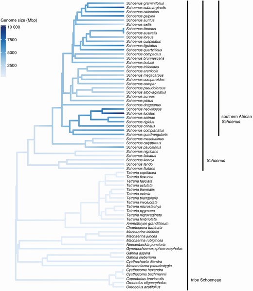
Mean holoploid genome size (Mbp) per species mapped onto the phylogeny of tribe Schoeneae. Only species with both genome size estimates and phylogenetic information are included in the figure. The estimation of maximum likelihood (ML) ancestral states was conducted with the R function ‘fastAnc’ (package ‘phytools’; Revell, 2012) and mapped onto the phylogeny with ‘ggtree’ (package ‘ggtree’; Yu et al. 2017).
Phylogenetic signal was absent in subtribe Schoeneae, Schoenus and the southern African Schoenus for both genome size and chromosome number (Fig. 2; Table 2). Estimates of Blomberg’s K were highest, but not significant, for tribe Schoeneae for both genome size (K = 0.070) and chromosome number (K = 0.037), and lowest for the southern African Schoenus (genome size: K = 0.025; chromosome number: K = 0.026; Table 2).
Estimates of phylogenetic signal calculated with Blomberg’s K.
| Variable | Taxonomic group | Blomberg’s K | P-value |
|---|---|---|---|
| Genome size | tribe Schoeneae | 0.070 | 0.598 |
| Schoenus | 0.067 | 0.607 | |
| southern African Schoenus | 0.025 | 0.835 | |
| Chromosome number | tribe Schoeneae | 0.037 | 0.458 |
| Schoenus | 0.035 | 0.673 | |
| southern African Schoenus | 0.026 | 0.730 |
Blomberg’s K was calculated with the function ‘phylosig’ in the R package ‘phytools’ v.0.7-80 (Revel, 2012). The significance of K is based on hypothesis tests composed of 1000 random simulations.
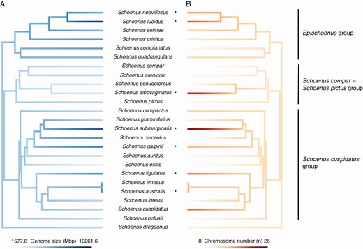
Mean holoploid genome size (Mbp) per species (A) and chromosome number (n: B) mapped onto the phylogeny of the southern African Schoenus. Only species with genome size and chromosome number estimates, as well as phylogenetic information are included in the figures. Species inferred as polyploid by ChromEvol are indicated by an asterisk. These two continuous characters were mapped onto the phylogeny with the R function ‘contMap’ (package ‘phytools’; Revell, 2012).
Ploidy inference
Of the 24 southern African species with available chromosome number estimates included in the ploidy inference analysis using the likelihood-based approach implemented in ChromEvol, seven were inferred as polyploids (Schoenus submarginalis, S. galpinii, S. australis, S. ligulatus, S. albovaginatus, S. neovillosus and S. lucidus: Supplementary Data Fig. S3). Four of these species were scattered throughout the S. cuspidatus group, one was inferred from the S. compar – S. pictus group and three were attributed to the Epischoenus group (Fig. S3).
Ploidy inference based on our genome size data provided further insights into the presence of polyploidy in southern African Schoenus, suggesting differences in intraspecific levels (i.e. diploid and polyploid in the same species) in five species (Supplementary Data Fig. S4). Of the five species with variation in intraspecific ploidy, the genome size data suggested three polyploids (Schoenus exilis, S. cuspidatus and S. pseudoloreus) in addition to the seven inferred by the ChromEvol analysis (Fig. S4). Furthermore, two species inferred as polyploid by ChromEvol (Schoenus submarginalis and S. ligulatus) also had diploid specimens based on our interpretation of the genome size data (Appendix S1, Fig. S4). All of the species with intraspecific variation in ploidy were scattered throughout the S. cuspidatus and S. compar – S. pictus groups (Fig. S4).
Relationship between genome size and chromosome number
Genome size was significantly positively correlated for all of the Schoenus (PGLS: estimate = 264.26, R2adj = 0.42, P < 0.001; Fig. 3A; Table 3) and for the southern African Schoenus clade (PGLS: estimate = 231.86, R2adj = 0.35, P < 0.001; Fig. 3B; Table 3). However, there was not a significant relationship between genome size and chromosome number when controlling for ploidy level (Fig. 3C; Supplementary Data Table S4), although there was a tendency for ChromEvol to infer those species with higher chromosome numbers to be polyploids regardless of their genome size (Fig. 3C).
Associations between chromosome number (n) and holoploid genome size (Mbp) for Schoenus and the southern African Schoenus clade, while considering phylogenetic relationships among species.
| Clade | Slope estimate | Slope standard error | t value | R 2 adj | lambda | PGLS P-value |
|---|---|---|---|---|---|---|
| Schoenus | 264.26 | 57.85 | 4.57 | 0.42 | 0.000 | <0.001* |
| southern African Schoenus | 231.86 | 61.66 | 3.76 | 0.35 | 0.373 | 0.001* |
| Clade | Slope estimate | Slope standard error | t value | R 2 adj | lambda | PGLS P-value |
|---|---|---|---|---|---|---|
| Schoenus | 264.26 | 57.85 | 4.57 | 0.42 | 0.000 | <0.001* |
| southern African Schoenus | 231.86 | 61.66 | 3.76 | 0.35 | 0.373 | 0.001* |
We conducted phylogenetic generalized least squares (PGLS) analyses with the function ‘pgls’ (R package ‘caper’ v.1.0.1; Orme et al., 2013). Significant relationships between variables (P ≤ 0.05) are indicated by an asterisk (*).
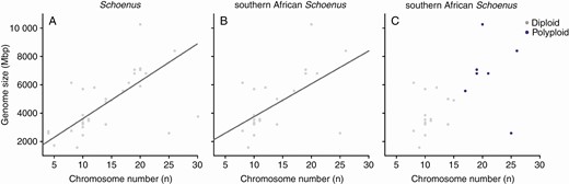
Relationship between chromosome number (n) and holoploid genome size (Mbp) for Schoenus (A), the southern African Schoenus clade (B) and the southern African Schoenus indicating ploidy levels as inferred by ChromEvol (C). All analyses considered phylogenetic relationships among species with phylogenetic generalized least squares (PGLS) with the function ‘pgls’ (R package ‘caper’ v.1.0.1; Orme et al. 2013). Significant relations (P < 0.05) between variables are indicated by solid regression lines. In C, diploids (D) are indicated in grey and polyploids (P) in purple.
Correlates of ploidy level and genome size evolution in the southern African Schoenus
After accounting for the other environmental variables in the ‘Extracted environmental’ dataset, polyploids had a higher probability of being associated with sites with lower annual precipitation (MCMCglmm: posterior mean = −2.27, pMCMC = 0.002; Table 4), higher precipitation seasonality (MCMCglmm: posterior mean = 46.73, pMCMC = 0.000; Table 4) and precipitation of the driest month (MCMCglmm: posterior mean = 455.76, pMCMC = 0.005; Table 4). These values were similar when S. albovaginatus (ploidy level unclear) was removed from the dataset (Supplementary Data Table S5). Results from the ‘Augmented extracted environmental’ dataset differed, with polyploids having a higher probability of occurrence on sites with higher annual temperature and precipitation seasonality, respectively (Table S6). The associations between polyploid and temperature in the coldest month, as well as temperature range, were negative (Table S6). This association signifies that lower values for both these variables were correlated with higher probabilities of polyploidy, while accounting for the other environmental variables in the dataset. Removing S. albovaginatus affected the results of the ‘Augmented extracted environmental’ dataset, as all six temperature and precipitation variables had significant associations with ploidy levels (Table S7). Specifically, polyploids had a higher probability of occurrence with higher annual temperatures, greater precipitation seasonality and increased precipitation of the driest month. In contrast, polyploids had a higher probability of occurrence when annual precipitation was less, when there was a narrower temperature range between the warmest and coolest months, and when temperatures of the coldest month were higher. Finally, there was no association between ploidy level and either N or P in the ‘Measured soil’ dataset (Table S8).
Summary results from MCMCglmm analysis with ploidy level (diploid or polyploid) as the response variable.
| Posterior mean | Lower 95 % confidence interval | Upper 95 % confidence interval | Effective sample size | pMCMC | |
|---|---|---|---|---|---|
| Intercept | −1805.16 | −5263.37 | 1410.30 | 82 377.70 | 0.245 |
| Elevation | −0.09 | −1.07 | 0.91 | 75 872.34 | 0.818 |
| N | −157.75 | −919.38 | 552.74 | 37 988.92 | 0.681 |
| P | 9.87 | −10.16 | 31.17 | 69 613.27 | 0.303 |
| Annual precipitation | −2.27 | −3.69 | −0.86 | 76 742.79 | 0.002** |
| Annual temperature | 102.69 | −1.26 | 206.31 | 79 952.43 | 0.052* |
| Temperature range | −52.45 | −107.16 | −0.01 | 79 307.26 | 0.056* |
| Precipitation seasonality | 46.73 | 21.64 | 71.72 | 73 770.72 | 0.000** |
| Temperature cold | −104.57 | −214.34 | 6.97 | 79 452.41 | 0.065* |
| Precipitation dry | 55.76 | 15.40 | 98.52 | 71 578.13 | 0.005** |
| Phylogeny | 210 312.00 | 0.00 | 586 938.00 | 55 740.00 | |
| Intraspecific ploidy | 8 125 100.00 | 0.00 | 27 299.00 | 90 000.00 |
The MCMCglmm analysis was performed with the function ‘MCMGglmm’ in the R package ‘MCMCglmm’ v.2.32 (Hadfield, 2010), considering phylogenetic relationships among variables (Phylogeny) and intraspecific ploidy (Intraspecific_ploidy) as random variables. ‘Temperature cold’ corresponds to the mean temperature of the coldest quarter and ‘Precipitation dry’ represents the precipitation of the driest month. Further details on the parameter settings for this analysis are presented in Table 1. Significant relationships between ploidy level and fixed variables (≤ 0.05) are indicated by two asterisks (**), whereas marginally significant relationships (≤ 0.10) are marked with a single asterisk (*).
Soil N was positively related to genome size for the ‘Extracted environmental’ dataset, but this relationship was marginal (MCMCglmm: posterior mean = −1.94, pMCMC = 0.050; Table 5). All other associations between genome size and the various environmental and geographical variables in this dataset were not significant (Table 5). Furthermore, there were no significant associations between either soil N or P and genome size based on the ‘Measured soil’ dataset (Supplementary Data Table S9).
Summary results from MCMCglmm analysis with genome size as the response variable.
| Posterior mean | Lower 95 % confidence interval | Upper 95 % confidence interval | Effective sample size | pMCMC | |
|---|---|---|---|---|---|
| Intercept | 7391.11 | −2180.14 | 17 144.53 | 3455.69 | 0.136 |
| Elevation | −1.22 | −4.49 | 2.05 | 3744.67 | 0.479 |
| N | 1997.45 | −58.16 | 4094.04 | 3336.74 | 0.050* |
| P | −1.79 | −69.00 | 69.02 | 3950.00 | 0.965 |
| Annual precipitation | −2.13 | −6.04 | 1.54 | 3950.00 | 0.275 |
| Annual temperature | 116.37 | −180.71 | 410.22 | 3773.19 | 0.446 |
| Temperature range | −67.91 | −213.38 | 99.44 | 3950.00 | 0.413 |
| Precipitation seasonality | 35.95 | −18.12 | 93.65 | 3950.00 | 0.207 |
| Temperature cold | −140.38 | −442.17 | 198.09 | 3762.80 | 0.401 |
| Precipitation dry | 6.28 | −85.91 | 104.57 | 3642.99 | 0.895 |
| Phylogeny | 4 199 422.00 | 1 623 473.00 | 7 378 529.00 | 3487.00 |
The MCMCglmm analysis was performed with the function ‘MCMGglmm’ in the R package ‘MCMCglmm’ v.2.32 (Hadfield, 2010), considering phylogenetic relationships among variables (Phylogeny) as a random variable. ‘Temperature cold’ corresponds to the mean temperature of the coldest quarter and ‘Precipitation dry’ represents the precipitation of the driest month. Further details on the parameter settings for this analysis are presented in Table 1. Marginally significant relationships between genome size and fixed variables (≤0.10) are indicated by an asterisk (*).
DISCUSSION
Using genome size and chromosome number estimates obtained for the southern African Schoenus, we show evidence of polyploidy in several species. We demonstrate associations between ploidy level and annual precipitation, as well as precipitation seasonality in this clade. In addition, we show a positive association between soil N and genome size based on the ‘Extracted environmental’ dataset. At a wider phylogenetic scale, we show that genome sizes in Schoenus (subtribe Schoeninae) are larger than those measured from species of the other seven subtribes of tribe Schoeneae, although chromosome number estimations do not follow the same pattern. Collectively, these results indicate the importance of combining chromosome counts with other types of data when determining ploidy levels in holocentric lineages.
Polyploidy in the southern African Schoenus
By sampling over half of the southern African Schoenus species, we show that polyploidy is probably relatively common throughout this lineage. Our results suggest that there are intraspecific differences in ploidy level (i.e. autopolyploidy) in Schoenus, similar to Kaur et al. (2012) who suspected one species in their New Zealand study of Schoenus to be of autopolyploid origin. We acknowledge that morphological species circumscriptions, such as those used to delineate the southern African Schoenus, are an important factor determining whether there are intraspecific differences in ploidy level, since polyploid lineages might not be visibly distinguishable from their diploid progenitors (Soltis et al., 2007; Husband et al., 2013). However, it would be impracticable to delineate species based on cytotypes in this clade due to the amount of variation in chromosome number and the lack of morphological characters associated with these differences. Further study involving genomic data is required to confirm the prevalence of allopolyploidy in the southern African Schoenus, although we suspect that specimens with intermediate morphologies (e.g. Schoenus auritus and S. cuspidatus intermediates), as well as having double the size of genome and number of chromosomes compared to nearby, morphologically similar species might be allopolyploids. Previous taxonomic work based on morphological characters has suspected hybridization resulting in allopolyploidy in this clade (Levyns, 1950, p. 124; Elliott and Muasya, 2020a), even though until recently this process was viewed as rare across the Cape region of southern Africa (Potts et al., 2018).
We inferred ploidy with ChromEvol, which uses both phylogenetic information and chromosome count estimations to determine whether species are diploid or polyploid. Other studies focusing on chromosome evolution in the Cyperaceae have also used this tool; however, their goals were to reconstruct ancestral chromosome numbers (Burchardt et al., 2020) and model the mode of chromosome evolution (Márquez-Corro et al., 2019) and not infer ploidy levels. Although we think that ChromEvol correctly inferred the ploidy level of most of the species that we included in the analysis, we are suspicious about the inferences made for one species. Genome sizes for S. albovaginatus were similar to those for other species in the S. compar – S. pictus group, whereas the chromosome number of this species was 2.5 times greater than the highest number for the other species in this group (Fig. 3C), suggesting a massive chromosome fragmentation event and not polyploidy as inferred by ChromEvol. However, this tool would have to consider other types of data (i.e. genome size estimations) for it to discriminate between these two processes. In addition, without considering other types of data, it is not possible to distinguish between aneuploidy sensu stricto (i.e. gain or loss of individual chromosomes: Blakeslee et al., 1920; Matzke et al., 1999) and chromosome fission/fusion, where the amount of genomic material remains relatively constant. The development of an approach that considers both changes in chromosome number and genome size would be beneficial in understanding complex chromosome evolution, such as occurs in holocentric lineages.
Our results demonstrate a positive relationship between genome size and chromosome number for both the southern African Schoenus, as well as the entire genus. A positive relationship between these two variables has also been shown in two other Cyperaceae genera: Carex (Lipnerová et al., 2013) and Eleocharis (de Souza et al., 2018). Of note, Lipnerová et al. (2013) illustrated how polyploidy drives this linear relationship in Carex, as polyploids have proportionally higher genome sizes and chromosome numbers compared to their diploid relatives. Our figure that incorporates the ploidy level of southern African Schoenus species (as inferred by ChromEvol) with their genome sizes and chromosome numbers (Fig. 3C) shows that there is a trend for taxa designated as polyploids to be in the top right-hand corner of the plot, which would help drive a positive relationship between the two variables.
At a wider phylogenetic scale, it is not clear how prevalent polyploidy is in the Cyperaceae, partially due to the complexities in confirming polyploidy in this holocentric family and a lack of comprehensive sampling. As massive chromosome fragmentation events might also lead to an approximate doubling of chromosome numbers, chromosome count estimates should be accompanied by another type of data that confirms that the quantity of genomic material in each cell has increased by about 2×, such as genome size estimates (e.g. Roalson, 2008; Zedek et al., 2010; Burchardt et al., 2020; Johnen et al., 2020), comparison of relative chromosome sizes (e.g. da Silva et al. 2010), and fluorescence in situ hybridization (FISH) and/or genomic in situ hybridization (GISH) approaches (e.g. da Silva et al., 2017; Johnen et al., 2020). Moreover, stomata measurements can also be used as a proxy in estimating relative genome sizes (e.g. Harms, 1968; Bureš, 1998), since a clear relationship has been shown between genome size and cell size (Beaulieu et al., 2008; Hodgson et al., 2010; Veselý et al., 2012). Although there has been an increase in the number of Cyperaceae taxa receiving cytological attention in the last decade, the prevalence of polyploidy across many genera in this large family remains unknown and understudied. Specifically, evidence of polyploidy in most of the 95 currently recognized genera in this family is lacking, with the exception of studies focusing on several of the larger genera (e.g. Schoenoplectus and Schoenoplectiella: Yano and Hoshino, 2005; Scleria: Yano and Hoshino, 2007; Schoenus: Kaur et al., 2012; Carex: Lipnerová et al., 2013; Rhynchospora: Burchardt et al., 2020). Numerous studies have demonstrated the occurrence of polyploidy in Eleocharis (e.g. Harms, 1968; Bureš, 1998; da Silva et al., 2010, 2017; Zedek et al., 2010; Johnen et al., 2020), whereas Carex has been the focus of many studies focusing on chromosomal fission and fusion, as well as chromosomal rearrangements (e.g. Hipp et al., 2009; Chung et al., 2012).
Relationships between ploidy/genome size and environmental correlates
Across the various analyses focusing on the environmental correlates of polyploidy, our results show that polyploids are more often associated with drier locations that have more variation in precipitation between dry and wet months. These results support the prediction that water deficits might be related to an increased prevalence of polyploidy, possibly through a greater production of unreduced gametes (Parisod et al., 2010). We are hesitant to draw too many conclusions from the results of these analyses, however, as they varied depending on the dataset (‘Extracted environmental’ versus ‘Augmented extracted environmental’) and whether S. albovaginatus was included in the data. Furthermore, the ploidy inference by ChromEvol might have also introduced errors in the classification of species as either polyploid or diploid, which would further influence how ploidy level is related to different environmental correlates based on our modelling approach. Although the climatic variables used in our study were based on measurements taken during a relatively short time frame (1979–2013), we view the data from this 35-year period to be representative of the current Cape climate and probably representative of the climate of the evolutionary history of the southern African Schoenus (see Hopper, 2009).
Supporting our predictions, we found a positive association between soil N and genome size. The relationship between both increased soil N and P levels and higher genome sizes has previously been demonstrated in fertilized grassland plots (Guignard et al., 2016). In addition, glasshouse experiments have demonstrated a more positive growth responses in polyploids compared to diploids under fertilized versus non-fertilized conditions (Walczyk and Hersch-Green, 2019). However, low levels of soil N were shown to favour diploids more than tetraploids after applying only soil N fertilizer to plots, but this relationship was not reversed for higher concentrations of N addition (Bales and Hersch-Green, 2019). Admittedly, our choice of total soil N as a predictor and not available N in the form of nitrate (NO3−) and ammonium (NH4+) is an over-simplification of the N requirements of plants. Nitrogen uptake in plants, including those in the fynbos of the Cape region of South Africa, is a complex and dynamic process varying through time, space and among species. For example, the spatial variation of soil NO3− and NH4+ has been shown to be greater than the variation of total soil N in fynbos, with fire complicating the situation as it can lead to large direct and indirect short-term impacts, including increased total soil N, NH4+ and NO3− (Stock and Lewis, 1986). Furthermore, species differ in their absorption and assimilation of soil NH4+ and NO3−, which can change throughout the season and the life cycle of a plant (Chapin, 1980; Stock and Lewis, 1984, 1986). Our results showing a connection between total soil N and genome size in the southern African Schoenus suggest that this relationship merits further attention, possibly by conducting a study focusing on different cytotypes of the same species grown at different concentrations of available soil N.
Larger genome sizes in Schoenus
The contrasting patterns in genome size we documented across tribe Schoeneae suggest that the underlying processes controlling this variable vary in importance across the lineage. Based on our limited data, genome sizes in subtribes Oreobolinae, Gahniinae, Gymnoschoeninae, Caustiinae, Lepidospermatinae and Tricostulariinae are relatively small, which might suggest a restricted role of polyploidy, similar to that documented in Carex (see Hipp et al., 2009; Chung et al., 2012), although more chromosome or other genomic data are required to make this conclusion. In contrast, variation and maximum genome sizes in Schoenus (subtribe Schoeninae) are much greater. Throughout other holocentric genera, polyploidy is a contributing factor to relatively large genome sizes in Eleocharis (Zedek et al., 2010) but not in Cuscuta (Neumann et al., 2021) or Luzula (Bozek et al., 2012); however, it is unclear how important it is in contributing to large genome sizes in other genera, such as Rhynchospora (Burchardt et al., 2020) and Drosera (Veleba et al., 2017). Furthermore, the role of repetitive DNA sequences in genome expansion/contraction and whether there has been a reduction in selection pressure constraining genome sizes in Schoenus compared to the other subtribes of tribe Schoeneae merits further study.
In summary, we show evidence of polyploidy both within and among species of the southern African Schoenus clade, suggesting that polyploidy in this lineage of holocentric plants is relatively common. In addition, our results suggest that differences in ploidy level in this clade are associated with short-term annual precipitation and precipitation seasonality. Although it is not clear whether polyploidy is a common process across the Cyperaceae, recent evidence suggests that it varies in prevalence across different tribes of the family. Further studies should incorporate several types of data when examining polyploidy in these and other holocentric plants because of the frequency of chromosomal fissions and fusions.
SUPPLEMENTARY DATA
Supplementary data are available online at https://dbpia.nl.go.kr/aob and consist of the following. Appendix S1: Additional sequences for the phylogenetic reconstruction. Appendix S2: Genome sizes of species from Schoeneae generated for this study. Appendix S3: ‘Extracted environmental’ dataset. Appendix S4: Samples included in the ‘Augmented extracted environmental’ dataset. Fig. S1: Mitotic chromosomes of Schoenus limosus and Schoenus cuspidatus × auritus (intermediate). Fig. S2: Holoploid genome sizes and chromosome number estimates across the eight subtribes of tribe Schoeneae. Fig. S3: Ploidy inference based on results from ChromEvol for the southern African Schoenus with available chromosome counts. Fig. S4: Ploidy inference based on results from ChromEvol for the southern African Schoenus with available chromosome counts. Table S1: Chromosome counts included in the study. Table S2: Summary of holoploid genome sizes across the eight subtribes of tribe Schoeneae. Table S3: Summary of chromosome numbers across the eight subtribes of tribe Schoeneae. Table S4: Relationship between chromosome number and holoploid genome size for Schoenus and the southern African Schoenus clade. Table S5: Summary results from MCMCglmm analysis based on the ‘Extracted environmental’ dataset. Table S6: Summary results from MCMCglmm analysis based on the ‘Augmented extracted environmental’ dataset. Table S7: Summary results from MCMCglmm analysis based on the ‘Augmented extracted environmental’ dataset (excluding ‘Schoenus albovaginatus’). Table S8: Summary results from MCMCglmm analysis with ploidy as the response variable (diploid/polyploid) for specimens with nutrients measured directly from the soil adjacent to their roots. Table S9: Summary results from MCMCglmm analysis with genome size as the response variable for specimens with nutrients measured directly from the soil adjacent to their roots.
ACKNOWLEDGEMENTS
We thank P. Jiménez-Mejías for his guidance in choosing appropriate fossil calibrations; W. Betz and M. Arens for field assistance; K. Nhlapo, D. Hattas and D. MacAlister for lab help and guidance; L. Horová and J. Šmerda for flow cytometric analyses; F. Zedek for analytical advice; and contributors to the iNaturalist project ‘Schoenus in southern Africa’. Computational resources were supplied by the project ‘e-Infrastruktura CZ’ (e-INFRA CZ ID:90140) supported by the Ministry of Education, Youth and Sports of the Czech Republic. New South African specimens included in this project were collected under CapeNature permit numbers CN35-28-4102 and 0028-AAA008- 00233; Province of the Eastern Cape Department of Economic Development, Environmental Affairs and Tourism permit numbers CRO 02/17CR and CRO 03/2017; Eastern Cape Parks & Tourism Agency permit number RA 0256; and South African National Parks permit numbers CRC/2016-2017/011—2016/V1, CRC/2017-2018/011—2016/V1 and ELLT/AGR/2019-2022/011—2016/V2. T.L.E. and A.M.M. conceived the study and contributed to field study collections. T.L.E. identified the specimens, conducted the chromosome counts, prepared the soil for analysis, analysed the data and prepared the first draft. P.B. managed the flow cytometric analyses. A.M.M. and P.B. provided input for subsequent drafts. The final manuscript was approved by all authors.
Funding
This work was supported by the University of Cape Town (Smuts Memorial Botanical Fellowship to T.L.E.; grant to A.M.M.); Fonds de recherche du Québec – Nature et technologies (FQRNT; to T.L.E.), International Association for Plant Taxonomy (grant to T.L.E.); Foundational Biodiversity Information Programme (FBIP) of the South African National Research Foundation (NFR: grant 104879 to A.M.M.) and the Czech Science Foundation (grant GA20-15989S to P.B.).
LITERATURE CITED
