


Abstract
Woody plants (trees and shrubs) play an important role in terrestrial ecosystems, but their size and longevity make them difficult subjects for traditional experiments. In the last 20 years functional–structural plant models (FSPMs) have evolved: they consider the interplay between plant modular structure, the immediate environment and internal functioning. However, computational constraints and data deficiency have long been limiting factors in a broader application of FSPMs, particularly at the scale of forest communities. Recently, terrestrial laser scanning (TLS), has emerged as an invaluable tool for capturing the 3-D structure of forest communities, thus opening up exciting opportunities to explore and predict forest dynamics with FSPMs.
The potential synergies between TLS-derived data and FSPMs have yet to be fully explored. Here, we summarize recent developments in FSPM and TLS research, with a specific focus on woody plants. We then evaluate the emerging opportunities for applying FSPMs in an ecological and evolutionary context, in light of TLS-derived data, with particular consideration of the challenges posed by scaling up from individual trees to whole forests. Finally, we propose guidelines for incorporating TLS data into the FSPM workflow to encourage overlap of practice amongst researchers.
We conclude that TLS is a feasible tool to help shift FSPMs from an individual-level modelling technique to a community-level one. The ability to scan multiple trees, of multiple species, in a short amount of time, is paramount to gathering the detailed structural information required for parameterizing FSPMs for forest communities. Conventional techniques, such as repeated manual forest surveys, have their limitations in explaining the driving mechanisms behind observed patterns in 3-D forest structure and dynamics. Therefore, other techniques are valuable to explore how forests might respond to environmental change. A robust synthesis between TLS and FSPMs provides the opportunity to virtually explore the spatial and temporal dynamics of forest communities.
INTRODUCTION
How individual trees and shrubs occupy 3-D space is a defining feature of forest ecosystem dynamics (Dı́az and Cabido, 2001; McDowell et al., 2020). Plant architecture, the physical form of a plant as derived from the balance between internal and external processes, is a central but often overlooked element of forest ecology and evolution (Barthélémy and Caraglio, 2007). Individual-level form and function, in combination with the environment, ultimately contributes to overall forest ecosystem level processes, determining the biodiversity found within them, as well as the regulation of energy, water and nutrient fluxes. There are still many unanswered questions regarding the mechanisms that give rise to observable patterns of biodiversity, form and function in forests worldwide (Givnish, 1999; Condit et al., 2006; Bohn and Huth, 2017). Elucidating the role of structure in these mechanisms is a crucial step in predicting the ecological and evolutionary responses of vegetation to forecasted climate change, deforestation or species invasions at the scale of forests and also at the scale of individual trees and shrubs (henceforth referred to as ‘woody plants’).
One way to characterize the relationship between biodiversity and the structure of forest environments is through the lens of structural diversity (Tews et al., 2004), which denotes ‘the physical arrangement and variability of the living and non-living biotic elements within forest stands’ (LaRue et al., 2020), and acts on its own as a good predictor of many ecosystem functions (Felipe-Lucia et al., 2018; LaRue et al., 2019). Recently, efforts have been made to formalize the role of structural trait diversity in forest ecology and evolution with the development of a ‘plant structural economic spectrum’ to complement the existing ‘wood economic spectrum’ and ‘leaf economic spectrum’ (Verbeeck et al., 2019).
Structural diversity is generated through spatially varying factors that determine the availability of microhabitats within the area, setting preconditions for the existence of different species with varying niche requirements (Svenning, 1999; Dymytrova et al., 2016). Spatially varying microhabitats arise from factors such as small-scale variation in soil properties (Matkala et al., 2020), landscape topography (Zuleta et al., 2020), hydrological features of the terrain (Francis et al., 2020), and the inflows and outflows of biologically active material (including plants, animals, fungi, microbes, nutrients) to and from the forest of interest (Honkaniemi et al., 2021).
Further structural diversity is generated (1) through dynamic 3-D growth and development of woody plants and other herbaceous vegetation within a forest stand and (2) through constantly changing environmental factors, such as weather, and a wide choice of unpredictable anthropogenic and natural disturbances (land use, global warming, wind, fire, snow, pest outbreaks, landslides etc.), as well as (3) through temporal changes in the inflow and outflow of biologically active material. The growth of woody plants alone causes temporal changes, because it alters individual plant architecture (3-D spatial arrangement of the plant structure), creating within-plant structural diversity through microenvironments within branches and foliage, i.e. due to different structural features (Escudero et al., 2017; Asbeck et al., 2019), self-shading (Ventre-Lespiaucq et al., 2016) or weather (Nock et al., 2016). Heterogeneous microenvironments inside a crown can thus alter growth habits (Koyama et al., 2020) and the functioning of foliage (Ngao et al., 2017; Curtis et al., 2019). Growth of individual plants changes the spatial structure of the whole forest stand (e.g. canopy layers, canopy cover, gap dynamics, tree size variation), and, in combination with the flow of dead material from woody plants to the ground, generates further changes in the structural diversity and choice of microhabitats available (Kaufmann et al., 2018). This results in the well-known natural succession of forest stands over decades (Boukili and Chazdon, 2017; Hilmers et al., 2018). In yet longer temporal scales, this results in evolution over centuries to millennia as biological adaptations to changing and often unpredictable growth conditions appear (Areces-Berazain et al., 2021).
Given all the constituents of structural diversity, it is clear that representative sampling of dynamically changing individual woody plant and forest characteristics is challenging. Even at the scale of individual woody plants, for instance in studies of the growth and architectural form of particular species, it can be challenging to explain the observations without information about the spatial structure of the growing site (Lintunen and Kaitaniemi, 2010; Kunz et al., 2019; Hildebrand et al., 2021), about the architectural structure and functioning of the individual itself (Posada et al., 2009; Kennedy 2010), and without information about the temporal dynamics that are likely in the typical growth environment (Ishii et al., 2018).
Traditional forest research can be labour-intensive and time-consuming. Detailed structural measurements of individual woody plants across a large stand have often been considered impossible and, instead, allometric or other structural relationships are used as proxies for multiple structural traits (Condés et al., 2020). Destructive sampling or special climbing constructions have been essential to reach the top of large trees (Barker and Pinard, 2001). In addition, a long time-series beyond a typical researcher’s career would be required to capture the full dynamics of individual and stand development over time.
Now there is a potential game changer: a combination of terrestrial laser scanning (TLS) and highly detailed functional–structural plant models (FSPMs) that mimic actual plants (e.g. Louarn and Song, 2020) Together, they provide a pair of tools that fulfil many prerequisites for addressing challenges with research questions related to the structural dynamics of forests. Terrestrial laser scanning, optionally complemented with scanning from unmanned aerial vehicles, is a method that enables capturing the full 3-D structure of a forest stand with close to centimetre-level detail in a short amount of time (Liang et al., 2016; Calders et al., 2020), including the identification of individual trees and their species (Xi et al., 2020), the ground vegetation (Muumbe et al., 2021) and the topography of the terrain (Diamond et al., 2020). Methods for collecting additional spectral information to estimate the state of various physiological processes within trees along with the structural scanning are also being developed (Junttila et al., 2021).
Functional–structural plant models, in turn, are models that aim to integrate the dynamic development of 3-D plant architecture, the associated physiological functions of the plant, and the simultaneous influence of external factors present in the growth environment (Fig. 1). As they operate with the 3-D architectural form of plants and plant stands, FSPMs are suitable for exploring the effects of different constituents of structural diversity on the dynamic behaviour of ecosystems. However, the applicability of FSPMs has so far been limited, much due to the amount of required data and high computational demands of the models; hence the existing models typically cover the spatial extent of just a few tree individuals (Sievänen et al., 2008; Zhang and DeAngelis 2020). On the other hand, one of the former limitations in the development of FSPMs, the availability of structural data for the construction and validation of models, is now changing as FSPMs are suited to directly utilize data provided by TLS, and use it to develop models that explore long-term dynamic processes within trees and stands (Sievänen et al., 2018).
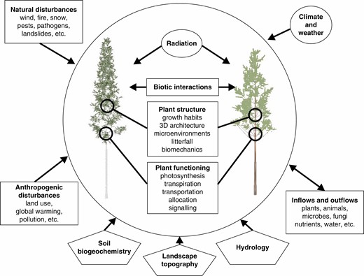
Structural heterogeneity of forest vegetation results from the interplay among multiple factors that influence structure and functioning of individual plants within forest stands over space and time. Current FSPMs largely focus on the encircled core of the system and consider the external factors with varying detail.
In this review, we will focus on recent developments of TLS and FSPMs, evaluate their current capabilities in data collection and modelling capacity, and evaluate the current and anticipated future applicability of these techniques in solving ecological and evolutionary questions when used in combination. In the first of the following three sections we will address the impact of plant architecture on vegetation modelling from the individual plant level to the forest level and the impacts of forest evolution. In the second section we will explore FSPMs and their three different sub-models: (1) physiological, (2) environmental and (3) architectural. In the third section we will evaluate the realm of TLS and the benefits that this field has to scale up FSPMs from an individual-level modelling paradigm to a community-level modelling paradigm. In the third section we also propose a potential TLS to FSPM workflow, evaluating the advantages and disadvantages of data collection and software involved. Lastly, we discuss the current and future synergies between TLS and FSPM for modelling forest communities.
MODELS OF INDIVIDUAL WOODY PLANT STRUCTURE AND FUNCTION
The form and function of woody plants, primarily trees, has captured the attention of biologists, mathematicians and artists alike for centuries. Since Da Vinci’s first mathematical formalization of tree structure, a large body of work has been dedicated towards understanding the mechanisms responsible for the array of tree shapes found across different habitats (Richter, 1970). Woody plants are dynamic organisms, composed of numerous self-similar and semi-autonomous parts, continually growing and developing from germination until death (White, 1979). In an effort to better understand the multitude of potential shapes, two botanists, Hallé and Oldeman, developed a qualitative system of describing different tree architectures found throughout tropical forests (Hallé et al., 1978). The concept of tree architecture eventually gave rise to the discipline of ‘architectural analysis’, which aims to investigate how underlying genetics and environmental adaptation contribute to ultimate tree form and function (Barthélémy and Caraglio, 2007).
Tree form and function have been studied using various hypotheses on how the extension growth, space-filling by the crown and thickening of already existing woody axes and root growth and the assimilation yield are related (West et al., 1999; Pałubicki et al., 2019). For example, regular scaling between woody axes and growing shoots or leaves has been observed and explained by several theories/models (Shinozaki et al., 1964; West et al., 2009). Such detail is sufficient for accurate characterization of crown and tree development (Sterck and Schieving, 2011), but since the physiological mechanisms for the processes are only partially known, the approach needs to rely on empirically determined or theoretical principles. Further, the parameter values of the scaling relationships vary with growing conditions and with tree crowns (Bentley et al., 2013).
Other approaches have also been used in the investigation of woody plant form and function: context-sensitive rules of development in crown dynamics can be applied that are related to physiology, including a carbon–nitrogen balance (Valentine and Mäkelä, 2012), photosynthesis (Peltoniemi et al., 2012) or transport of carbohydrates within the crown (Nikinmaa et al., 2013). Alternatively, rules can be defined by self-organization in branch growth (Pałubicki et al., 2009). It has also been argued that the crown development actually follows resource optimization (Givnish, 1984; Mäkelä et al., 2008; Sterck and Schieving, 2011; Franklin et al., 2020). Understanding the mechanisms of individual resource partitioning in woody plants and how this influences the 3-D shapes we see in nature underpins the overall structure of forests. One important area of active research is the accurate estimation of above-ground biomass (AGB) in forests globally, especially in the context of rapidly changing environments (Brienen et al., 2015). This inevitably relies on how well carbon allocation towards the different woody plant organs can be quantified. Formalized tree allometric models have been widely used to estimate carbon stocks and balance in forests (Chave et al., 2005, 2014). Whilst this is important for practical management and conservation, predicting future states of individual trees and their relative contributions to AGB requires further investigation of the driving processes of individual form and function in the context of their respective communities.
Models of forest communities
Unravelling the mechanisms of woody plant form and function in forest communities, across different habitats, is crucial for furthering ecological theory, designing forest management plans and informing global land surface models (Franklin et al., 2020; Ruiz-Benito et al., 2020). However, the precise mechanisms that determine form and function of woody plants in forest environments have been largely overlooked in ecology until recently (Malhi et al., 2018). In addition to the barriers in collecting data on forest communities (i.e. the impracticality of dealing with large, long-lived individuals and destructive harvesting), which make woody plants less than ideal subjects for experimental investigation, there remain a number of barriers in how organisms with a sessile but highly adaptive growth habit are sampled. Many of the methods typically used in ecology, such as counting individuals of varying age and size class, are insufficient to explain the broad intraspecific and interspecific variation found in forests (Harper, 1977, 1980). Furthermore, community ecology research had been dominated by a ‘mean field theory’ approach for years, which emphasizes differences between co-occurring species rather than differences between individuals of the same species (McGill et al., 2006; Weiher et al., 2011).
It is only in the last decade that efforts have been made to revisit the importance of intraspecific variation as a driver of community assemblage and integrate it into community ecology (Violle et al., 2012; Hildebrand et al., 2021). This is particularly pertinent for forests, where potentially high levels of intraspecific variation but low levels of interspecific variation can occur, as individuals converge on a common limiting resource (MacFarlane and Kane, 2017). Comparisons between mean field theory approaches and spatially explicit individual-based models (IBMs) have indicated that the spatial distribution of individuals in a forest can better explain ecosystem function and biomass production seen in nature, as opposed to a mean-field approach at the community level (Pacala and Deutschman, 1995). Woody plants interact on a local rather than a global scale, and therefore individual functional variability and growth strategies have clear implications for models at higher levels of ecological organization, such as dynamic global vegetation models (DGVMs) (Scheiter et al., 2013). Spatially explicit IBMs have been used for decades in plant and forest ecology and forest science to better address heterogeneity amongst individuals in a community (Houston et al., 1988; Grime, 2006). These models are able to capture many key elements of plant competition, such as individual variation and heterogeneous distribution of resources (Fisher et al., 2017). However, they traditionally lack a mechanistic explanation of these phenomena (Canham et al., 2004). Moreover, these models do not interpret how individuals modify their local environment through 3-D adaptive behaviour (Grime, 2006; Brooker et al., 2008).
Moving away from ‘mean’ approaches, whether that be in practical vegetation modelling or the development of paradigmatic theories, is paramount to fully exploring the drivers of forest structure and dynamics. In summary, a model with an applicability for diverse studies of evolutionary and ecological questions involving woody plant communities should possess the following properties in order to account for the role of vegetation structure and function in the processes investigated: it should account for the main processes of plant development (Sorrensen-Cothern et al., 1993; DeAngelis 2018): (1) resource capture as a response to the immediate environment; (2) allocation of growth that results from resource capture to the development of the 3-D crown architecture; and consequently (3) modification of the immediate environment, described as a 3-D distribution of the resource flux. The model should also have modules that are sufficiently easily parameterized for (4) physiological processes (growth engine) and (5) morphological development (crown architecture) for different species. It would be beneficial if (6) different plant parts (organs) could be singled out (e.g. node, internode, leaf, bud) without simplified representations, such as spatial distributions. Further, (7) the model should be able to cover the whole life span of the woody plant, from seedling to maturity, including some measure of fecundity and mortality. (8) Spatially explicit individual-based simulations of a sufficiently large plant community are necessary. (9) An easy link with structural measurements would be useful, and finally (10) the model should be able to incorporate temporal variation.
Numerous plant community models are capable of fulfilling at least some of the above criteria. For example, process-based models can describe growth derived from physiological processes interacting with the environment (criteria 2 and 4 above) and have been used successfully for many years in agronomy (Bouman et al., 1996; Marcelis et al., 1998) and forest sciences (Mäkelä et al., 2000). However, they lack the 3-D spatial and structural information of individuals which ultimately modifies fine-scale resource capture and growth in forest environments. Alternatively, gap models (Botkin et al., 1972) include detailed life cycles and can differentiate between different species (criteria 1 and 5), which is beneficial for modelling plant community interactions. However, neither the specific 3-D form of individuals nor their spatial distribution in a simulation (criteria 2, 3 and 8) is explicit. There also exist ‘cohort-based models’, which act as an intermediary between IBMs and DGVMs, whereby plants are grouped by age, size or functional types (Fisher et al., 2017). These models are not as computationally heavy as IBMs but reduce the resolution of functional diversity (Fisher et al., 2010). The placement and specific architecture of individuals within a community and their relative distances to each other are important factors for determining the strength of interactions between neighbours. Individual woody plant structure determines forest community structure, but this is itself determined by the structure of neighbouring woody plants. Models without 3-D structural variation will not capture within- and between-plant microenvironments, therefore losing information regarding fine-scale patterns of form and function in heterogeneous environments.
Indeed, many community models have been developed which account for forest structure and spatial heterogeneity including SORTIE (Pacala et al., 2011), LPJ-GUESS (Smith et al., 2014), ED/ED2 (Moorcroft et al., 2001) and FORMIND (Köhler and Huth, 1998). These models have been able to answer a number of ecological and evolutionary questions with regard to forest structure and dynamics, including the effect of shading and crowding on neighbours (Canham et al., 2004). Nevertheless, all these models have a simplistic representation of 3-D structure, omitting explicit branching and growth asymmetry, which can impact the presence of microenvironments. Indeed, high-level vegetation models including landscape forest models (Mladenoff, 2004) and DGVMs (Prentice et al., 2007) rely on assumptions derived from plant community models, and thus it is important to investigate and evaluate the relative 3-D structural contributions of individuals in forest communities and how these ultimately impact vegetation assembly and dynamics (Zhang and DeAngelis, 2020).
Evolutionary models
Evolutionary woody plant and community models typically operate with simplified or purely theoretical communities, and often focus on identifying different adaptive strategies and differences in niche utilization that are suggested to enable the development and coexistence of diverse woody plant species (Lamanna et al., 2014). In recent years, these models have included the performance of individual plants that are growing in spatially explicit positions within a model system (May et al., 2015; Coelho and Rangel, 2018; Wickman et al., 2019). An accumulating line of evidence suggests that there can exist multiple alternative functional–structural tree designs that share an equal value of a fitness measure (Dias et al., 2020), which is in line with the ideas of Pareto optimal plant design (Farnsworth and Niklas, 1995; Conn et al., 2017) and the neutral theory of biodiversity (Hubbell, 2001). For example, Falster et al. (2017) demonstrated that the inclusion of few mechanistic details in a spatial forest model enabled diverse competitive coexistence in a manner that closely resembled the situation where different plant species are functionally identical. Xiao et al. (2007) concluded that there is no single evolutionarily stable height strategy for a plant population. Kennedy (2010) showed that alternative branch morphologies can compensate for water stress while simultaneously maximizing carbohydrate gain.
While increasing realism may sound beneficial, it can also easily lead to an added amount of model uncertainty due to practical challenges in specifying numerous parameter values with sufficient reliability. Equal performance of alternative designs also suggests that increasing the level of detail beyond a certain point may not produce further changes in model predictions, if the model simply depicts these alternative designs. However, detailed analyses of the roles of different functional and structural traits can be warranted in situations such as the need to select plants with favourable trait combinations for specific purposes (Picheny et al., 2017). Hidden differences between alternative trait combinations may also become realized if the environment changes.
Franklin et al. (2020) suggested that the potential problems of model complexity in vegetation models could be circumvented by applying only three evolutionarily justified organizing principles to predict individual variation: natural selection, self-organization and entropy maximization. There are already examples where self-organizing principles alone can produce a high diversity of tree forms (Pałubicki et al., 2009) and simulate long-term dynamic development of forest vegetation over a wider topographically variable area (Makowski et al., 2019).
GENERAL FEATURES OF FSPMS
Functional–structural plant models are complex 77models, but in light of increasing data availability, they now have the potential to be useful as tools for investigations on forest communities from the dynamic and evolutionary point of view and fulfil all the desired criteria outlined above (Louarn and Song, 2020). The FSPMs appeared in the mid-1990s with the aim of unifying classic process-based plant models with geometric models (Sievänen et al., 2000; Godin and Sinoquet, 2005). FSPMs differ from earlier models of plant growth by considering an individual plant as a collection of semi-autonomous, interconnected elementary units. Metabolites allocated to those units are determined through availability derived from metabolic processes in the context of their environment (Fig. 2). The resulting model is structurally and functionally realistic and expresses highly responsive behaviour in relation to the prevailing growth conditions, which gives insight into the nuances of 3-D structure otherwise overlooked in other modelling techniques (Fig. 3). A good sample of previous research into FSPMs and related topics can be found in special issues of New Phytologist166 (3), 2005; Functional Plant Biology 35, 2008; Annals of Botany101 (8), 2008, 107 (5), 2011, 108 (6), 2011, 114 (4), 2014; 121 (5), 2018 and 126 (4), 2020; and Ecological Modelling290 (1–2), 2014.
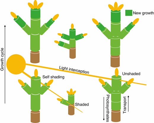
A schematic representation of how an FSPM interacts with the environment with multiple individuals simulated. Here, an environmental sub-model determines the amount of light available for photosynthesis. The overall structure of the plant determines how much light can reach different parts of the plant, which is then utilized by the physiological sub-model to calculate metabolites used for the next growth cycle. In multi-individual simulations, light is intercepted by neighbours, thus reducing resource capture.
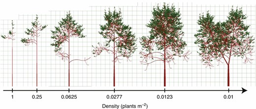
Example of FSPM function under changing environmental factors (Cournède et al., 2008). In this case, the density of individuals decreases from left to right, highlighting the impact of growing conditions on tree structure.
Table 1 shows a sample of FSPMs applied for simulation of growth of woody plants. The most popular purpose of model construction is in the realms of horticulture and agronomy. This is understandable since the FSPMs are well suited for increasing understanding of resource flux to desirable products and simulation of management effects such as pruning. A clear driver in the development of these models is to improve our understanding of the interplay between resource acquisition and architectural development. Notably, these models are all based on resource capture of aerial parts only. Some models include roots but only as a passive part of the plant. There are numerous functional–structural models of root systems (Barczi et al., 2018; Schnepf et al., 2018) but none of them have been linked to the models listed here. Some of the models have been realized using a dedicated software for FSPMs. Notable examples of such software include AmapSim (Barczi et al., 2018), GroIMP (Hemmerling et al., 2008), Virtual Laboratory/L-studio, (http://www.algorithmicbotany.org/virtual_laboratory/; Prusinkiewicz, 2000) and OpenAlea/OpenAleaLab (https://team.inria.fr/virtualplants/software/; Pradal et al., 2008). Amongst the many FSPMs that have been developed, significant variation can be found in their implementation. Nevertheless, FSPMs always feature three main components or sub-models: a physiological model, an environmental model and a structural model.
An overview of FSPMs that simulate dynamic growth of woody plant species. In addition to the publications, information about the models on the site www.quantitative-plant.org has been utilized. N.i., no information available; UML, Unified modelling language
| Model | Species | Time step/time range | Parameter input | Multi-plant simulation? | Programming language/software | Open-source | Purpose/comment | Citation |
|---|---|---|---|---|---|---|---|---|
| ECOPHYS | Poplar | Hour/several years | Biologically derived | Yes | C++ | N.i. | Disentangling growth factors | (Host et al., 1996, 2008) |
| GreenLab | Generic/beech, Mongolian pine | Can choose/decades | Biologically derived/Stat. fitting | Yes | Matlab, Java, Cpp, Scilab | Upon request, freeware | Resource capture, plant architecture | (Cournède et al., 2008; Letort et al., 2008; Wang et al., 2012) |
| GroIMP (Beech) | Generic/beech | Year/decades | Biologically derived | Yes | GroIMP, XL (Kniemeyer and Kurth, 2008) | Yes | Demonstration of software | (Hemmerling et al., 2008) |
| IMapple | Apple tree | Hour/decades | Biologically derived | Yes | C# | N.i. | Horticulture | (Kang et al., 2016) |
| LIGNUM | Pine, maple, poplar/generic | Year or growth cycle/decades | Biologically derived | Yes | C++, L+Cc (Vos et al., 2007) | Upon request, GitHub | Study of crown development | (Perttunen 2001; Sievänen et al., 2008; Lu et al., 2011) |
| L-Peach | Peach tree | ~1 d/several years | Biologically derived | Focus is one tree | L-studio (Prusinkiewicz, 2000) | Upon request | Horticulture | (Allen et al., 2005; Lopez et al., 2008; Da Silva et al., 2014) |
| Macadamia model | Macadamia tree | Day/growing season | Biologically derived | No | L-studio (Prusinkiewicz, 2000), L + C (Vos et al., 2007) | N.i. | Horticulture, proof of concept | (Auzmendi and Hanan 2020) |
| MAppleT | Apple tree | ~1 d/several years | Biologically derived | Focus is one tree | L-Py (Boudon et al., 2012), OpenAlea (Pradal et al., 2008) | Yes | Horticulture | (Costes et al., 2008) |
| QualiTree | Peach (fruit trees) | Day | Biologically derived | Yes (canopies as ellipsoids) | UML (object technologies) | N.i. | Horticulture, fruit development | (Lescourret et al., 2011; Mirás-Avalos et al., 2011) |
| Radiata pine | Pinus radiata | Month/several years | Biologically derived | No | Basic | N.i. | Silvicultural decisions | (Fernández et al., 2011) |
| Sterck model | Generic deciduous | Day/decades | Biologically derived | No | N.i. | N.i. | Ecological–evolutionary problems | (Sterck et al., 2005; Sterck and Schieving 2007) |
| V-Mango | Mango tree | Day/several years | Stat. fitting/Biologically derived | No | L-Py (Boudon et al., 2012), OpenAlea (Pradal et al., 2008) | N.i. | Horticulture | (Boudon et al., 2020) |
The main focus of the FSPM studies has been in the responses of single plants, either isolated or as a part of a plant community. If they have been part of a plant community, the effect of other plants has been modelled assuming some sort of homogeneity of the surrounding canopy. For example, Sterck et al. (2005) assume the surrounding canopy be characterized by its height and a homogeneous leaf distribution. Nevertheless, in spite of the predominant focus on individuals of FSPM tree applications, five of the 12 models listed in Table 1 are capable of simulating interacting tree individuals, i.e. scaling up from elementary units to tree community. Host et al. (2008) used the ECOPHYS model (Table 1) to simulate the growth over 8 years of individual aspen and Populus trees on a patch of 64 trees with an hourly time step. They observed how the growth differed between various clones for which the parameters of e.g. leaf-level light interception, carbon allocation, canopy architecture and phenological events had been determined. Cournède et al. (2008) simulated the effect of interplant competition for light and density on interacting individual trees in heterogeneous conditions using the GreenLab model (Table 1). Hemmerling et al. (2008) showed a simulation using the model GroImp (Table 1) of a landscape consisting of 700 individual beech and spruce trees for 11 years with an annual time step when the trees were interacting through radiation interception.
Computational requirements are no longer a major obstacle in the development of FSPMs at the community level. Taking the LIGNUM model (C++ implementation, Sievänen et al., 2008) as an example of computational requirement of multitree simulation, a rough estimate is as follows. The elementary units tree segment and bud can take 300 and 200 bytes, respectively. A tree with 50 000 units will consume 25 megabytes of memory. Extending this to 3000 trees (per ha) the memory requirement would be ~75 gigabytes. The second memory requirement comes from environmental modelling. One way to represent the growth space of plants is to discretize it to cubic volume elements using voxel space. For example, in the LIGNUM model, the individual elementary cubic element (a voxel), requires ~300 bytes. Assuming a voxel with 20 cm side length (roughly the size of an elementary unit tree segment) and the requirement for a 1-ha forest plot 40 m high, the number of voxels would be 50 million. This amounts to a roughly 15 gigabyte memory requirement for the voxel space.
A modern high-performance computing system can have hundreds of gigabytes or even terabytes of available memory (see examples at docs.csc.fi computing environment). Therefore, the large number of elementary units does not create an insurmountable computational obstacle as long as physiological processes can be computed in linear time, O(n), in terms of elementary units, as is the case in most of the models in Table 1, including the calculation of light transmission in canopy or tree crowns, for example, with the aid of voxel space (Sievänen et al., 2008). These examples indicate that the FSPMs are capable of simulating heterogeneous natural forests as interacting individual trees.
Major strides have been made in the physiological models, the environmental model and the structural model, particularly for non-woody plants, namely, the development of state-of-the-art light models (Dieleman et al., 2019), below-ground extensions of 3-D architecture (Barczi et al., 2018; Schnepf et al., 2018) and numerous physiological advances (Louarn and Song, 2020). So far, FSPM development has been largely dedicated towards modelling crop products: for example, grapes (J. Zhu et al., 2018; Schmidt et al., 2019; Prieto et al., 2020), tomatoes (Sarlikioti et al., 2011; Dieleman et al., 2019; Vermeiren et al., 2020), soybeans (Coussement et al., 2020; Song et al., 2020). The development of FSPM components in agronomy has been pivotal to the extension and improvement of FSPMs in general (Vos et al., 2010; de Reffye et al., 2021), but careful consideration must be taken when applying these models to ecological and evolutionary questions. For example, many agronomy-based FSPMs target fruit production (Table 1) and thus include detailed source–sink components that may be unnecessary for modelling natural forest stands (Allen et al., 2005). It is also worth noting that agronomy FSPMs often simulate growth and development in optimum environments, without any nutrient, water or light shortages (Auzmendi and Hanan, 2020), which is far removed from natural conditions. In short, each sub-model (environmental, structural and physiological) must be evaluated in turn to ascertain trade-offs between reality, generality and simplicity at larger spatial and temporal scales.
Physiological sub-models
The modular nature of FSPMs means that almost any physiological models (empirical or mechanistic) can be included and exchanged depending on the research question. Whilst this has benefits in testing and exploring a range of theories, it can quickly become overwhelming for non-experts. The growth and development of woody plants can be split into two categories of physiological processes: the ‘fast processes’ of photosynthesis and respiration and the ‘slow process’ of carbon allocation. Carbon is assimilated through photosynthesis and allocated either towards new growth or maintenance, whilst carbon losses occur through respiration and senescence. Photosynthesis has been represented in FSPMs in a number of ways, including implicit models (Mäkelä and Hari, 1986), empirical models (Le Roux et al., 2001) and biochemical models, notably the Farquhar–von Caemmerer–Berry (FvCB) model for C3 photosynthesis (Farquhar et al., 1980; von Caemmerer and Farquhar, 1981), which has been scaled up for whole canopies in Medlyn et al. (2003). Biochemical models have the added benefit of representing instantaneous responses at small time steps of minutes and hours, which may be beneficial for particular studies, for example in modelling fast-growing species (Lu et al., 2011). However, these short physiological time steps may not be necessary, or appropriate, for modelling forest structure and dynamics at larger spatial and temporal scales.
Notably, most of the FSPMs listed in Table 1 either ignore acclimation or prescribe fixed parameter values for each specific species. However, vascular plants are known to adapt their ‘fast’ physiological processes depending on their environmental conditions (Walters, 2005). For photosynthesis, a mechanistic approach, such as that employed by the P-model (Stocker et al., 2019) may be more appropriate for simulating the acclimation of photosynthesis over time. Here, an optimality-based theory is used to predict the acclimation of leaf-level photosynthesis to its environment. Moreover, a recent global analysis of forest production efficiency by (Collalti et al., 2020) observed that respiration rates varied with temperature far less steeply than observed in short-term responses, indicating acclimation over time. ‘Fast’ physiological processes in FSPMs are usually based on these instantaneous responses and it will be important in future development to consider the impact of this aspect on simulations at the scale of weeks, months and years. In the FSPM modelling paradigm, which is based on the concept of a plant’s adaptability to its local environment, it is imperative not to underestimate the importance of acclimation in basic physiological responses. Some areas to consider are CO2 acclimation as implemented in mCanopy-soybean (Song et al., 2020) or the light acclimation simulations of sugar maple trees in LIGNUM (Posada et al., 2012).
The ‘slow’ process of carbon allocation towards new growth and maintenance of existing organs is particularly important in FSPMs, but also one of the least well understood. Carbon allocation methods are difficult to compare between FSPMs because different models employ different groupings of parts (Zhang and DeAngelis, 2020). Most FSPMs include a carbon allocation model based on the pipe model theory (PMT) proposed by Shinozaki et al. (1964) over half a century ago (Godin, 2000; Le Roux et al., 2001; Lehnebach et al., 2018). Whilst this model provides a useful framework for investigating functional–structural relationships, many of its assumptions are outdated. Notably, in their comprehensive review of the PMT, Lehnebach et al. (2018) find that the property of sapwood area preservation is almost never valid, and that the ratio of leaf mass to a cross-sectional area of sapwood can vary greatly depending on internal and external properties. As an alternative, the authors suggest an additional model step not included in the PMT, which robustly quantifies foliage and sapwood partitioning regardless of species, age or stand condition. A broad uptake of such methods could be useful for comparing between FSPM models, particularly with regard to how carbon allocation is represented in models of herbaceous and woody plants. Furthermore, it permits explaining potential physiological adaptations found between individuals in a given forest community. It is worth noting that physiological sub-models of FSPMs are one of the greatest contributors of model complexity and still one of the most difficult to parameterize effectively, so a move towards simpler physiological sub-models would be greatly beneficial to FSPMs, particularly when applied to natural, multitree scenarios.
Environmental sub-models
Simulations of realistic local environmental conditions are a key determinant of how woody plants adjust to external processes. In FSPMs there are many ways to represent environmental conditions and these methods come with varying levels of reality and detail. A select few FSPMs have been able to capture detailed below-ground processes in herbaceous plants, notably C-Root Box (Schnepf et al., 2018), but the majority of FSPMs focus on above-ground processes. Thus, in terms of resource capture, light conditions are fundamental to understanding how individuals optimize form and function within their respective communities. Recent FSPM studies have indicated that light competition reduces individual plant defence against herbivory (de Vries et al., 2018, 2019). In addition, Douma et al. (2019), have shown that it is not only the quantity of light that contributes to plant defence, but also the quality of available light.
Thus, modellers must evaluate the potential options for representing an accurate light environment when developing FSPMs and scaling up from organ level to a forest patch by simulating the growth of individual trees. As the development of tree individuals takes place in terms of a collection of elementary units without simplifying assumptions of crown shape (if it was, it would be contrary to the idea of FSPMs), it is not easy to make use of stand-level simplifications in the calculation of radiation conditions. Rather, the analysis of radiation conditions needs to be made on the basis of actual positions of all individual shading units (foliage) and it is a computationally complex problem (Host et al., 2008). Although computers have advanced rapidly in recent years, the choice of light model can add a significant computational burden to the overall FSPM so trade-offs are inevitable.
Most methods of light simulation involve computing how much photosynthetically active radiation (PAR) is intercepted or absorbed by plant structural elements. To speed up radiation calculations, spatial discretization, such as the method of voxel space (Li et al., 2018), or some other means, like techniques based on Monte Carlo sampling in path tracing (Cieslak et al., 2008), can be applied. Alternatively, shadow propagation (Pałubicki et al., 2009) has been used, which is a fast approach to compute a coarse estimate of the exposure of each bud to light. In this approach the space is divided into a grid of voxels each with associated shadow value. Each plant segment occupying a particular voxel creates a pyramidal penumbra at the voxels underneath. All segments are sequentially processed to produce a 3-D grid of accumulated shadow values.
More recently, with improved parallel processing and the use of graphics processing units (GPUs), it has become possible to model detailed absorption, transmission and reflectance for the full light spectrum using ray-tracing models (Henke and Buck-Sorlin, 2017). A normal forward ray-tracing is based on the point of view of the radiation source (sky). This means that the rays from the source are traced to the elements of interest (i.e. leaves, buds, branches). However, this approach becomes problematic when the number of elements becomes large, because to sample them sufficiently and accurately requires a very large number of rays that sample the incoming radiation. Even then, there can be large errors in individual elements. The idea of reverse ray-tracing is to change the point of view from the radiation source to the entities themselves. Thus, the rays from every element are traced to the source, which ensures that each element is sampled properly and the errors are bounded. This approach has been used in a number of static FSPMs, including Helios (Bailey, 2018, 2019), and the FSPM generation platform GroIMP (Kniemeyer and Kurth, 2008; Hemmerling et al., 2008).
Architectural sub-models
One of the most widely known and commonly used methods of representing the 3-D structure of woody plants is through Lindenmayer systems, otherwise known as L-systems (Prusinkiewicz, 2000). L-systems are parallel rewriting strings that act on sequences of symbols. Woody plants can be represented by an L-system with an alphabet of symbols and a set of rewriting rules, known as productions. Each symbol in the alphabet represents a distinct botanical unit, such as buds, leaves or flowers. This system of rewriting allows for dynamic growth rather than just a static configuration of plant architecture in space. Numerous FSPMs use L-systems directly or software based on them, such as L-studio, L + C and L-Py (Table 1) to define plant structure. Creating successful L-systems that reflect realistic plant forms is an art in itself (Prusinkiewicz, 2004). It can quickly become laborious when multiple species with different growth habits, or individuals of different ages, need to be defined. Parameterizing L-systems in an informative way requires many structural parameters, which were difficult, if not impossible, to attain until the recent application of TLS technology to forest communities.
THE REALM OF TLS
In recent years, TLS has emerged as a revolutionary tool for measuring above-ground 3-D tree architecture and forest structure (Malhi et al., 2018; Disney, 2019; Calders et al., 2020). TLS is a ground-based remote sensing method of determining distance and is one of a wider choice of laser scanning techniques that provide often complementary information for different measurement scales and research purposes (Beland et al., 2019). Here, we consider TLS to also cover scanning from unmanned aerial vehicles capable of accessing the upper parts of the canopy (Slavík et al., 2020). There are numerous TLS instruments available commercially, and whilst they vary greatly in their specifications, they all function in the same way, by emitting a laser light onto a 3-D object and measuring the distance to the object. Three-dimensional representations, called point clouds, can then be generated based on the distances and directions of the laser beams. The potential benefits of this technology for elucidating forest structure and dynamics can hardly be overstated. TLS is a non-destructive technique that can produce measurements to within even millimetre accuracy, depending on the equipment used, without the need to fell trees. This significantly reduces the time required for taking detailed measurements of individuals and leaves the habitat intact for potential resampling at a later date. As TLS technology matures, so does the ability to scan larger areas with excellent resolution. The large quantities of high-accuracy structural data provided by TLS are invaluable for elucidating the underlying mechanisms of individual tree form and thus the whole-forest organization. Despite the promises and potential, the application of TLS to questions in forest ecology and evolution is still in its early days. In a recent review, Malhi et al. (2018) outline a number of areas suitable for testing and extending ecological theory on tree form and function in the context of TLS, including seed dispersal, structural mechanics and resource distribution. The opportunities are indeed exciting; however, tackling such theoretical questions with TLS requires careful coordination of elements spanning many disciplines.
In practice, TLS is time-efficient in relation to the gained precision and is easy to use; however, there are a number of nuances that must be taken into consideration to ensure overlap of practice between researchers. Some challenges will be present regardless of the equipment used or environmental conditions, which include, but are not limited to, occlusion, leaf and wood separation, irregularity of form and validation. Many of the commercially available TLS instruments are able to reduce common difficulties associated with scanning individuals, stands and large areas of mixed-species forests. The potential to test and further expand ecological theory stems largely from the ability to gain an accurate representation of how organs of a tree are arranged in 3-D space and how multiple trees in this space are arranged relative to each other. Similar to choosing the correct environmental and physiological elements to include when creating FSPMs, correctly planning both the data collection and data processing prior to beginning a project is key to maximizing the benefits of TLS. If all the trees in a forest plot are targeted, Wilkes et al. (2017) suggest a sampling grid of 10 m × 10 m in dense areas and 20 m × 20 m in open areas to produce a good-quality point cloud that effectively resolves higher-order branches down to a few centimetres in diameter in up to 30 m canopies. If individual woody plants are targeted, the sampling grid can be designed on a case-by-case basis to maximize the visibility of the individual.
A highly important use of TLS has been in quantifying AGB. Estimating AGB is crucial to our understanding of carbon stocks and fluxes but has been plagued by systematic error due to the difficulty in obtaining manual measurements, bias towards temperate regions and an over-reliance on allometric scaling equations. New TLS-derived measurements have deconstructed previous assumptions about AGB estimates and challenged the validity of many of the widely used allometric scaling equations (Disney et al., 2018). Notably, TLS estimates of AGB are free from the constraints of allometric models and can thus provide well-justified levels of uncertainty. Estimates of AGB derived from TLS tend to perform well in a number of scenarios, including tropical and urban environments; however, it should be noted that it is not a mature enough tool to be used as a standalone methodology (Wilkes et al., 2017; Lau et al., 2019). Currently, measurements from destructive harvests are frequently required to validate AGB estimates from TLS. It is also noteworthy that allometric models can be refined towards more flexible functional models using the type of data that is available from TLS (Kaitaniemi et al., 2020; Kaitaniemi and Lintunen, 2021). Alternatively, quantitative structural models (QSMs), which are a hierarchical collection of cylinders (Fig. 4), can be used to compute an array of detailed structural tree metrics, including AGB. There are published and freely available methods to reconstruct QSMs from TLS data; these include TreeQSM (Raumonen et al., 2013; Calders et al., 2015a; Raumonen, 2020), SimpleTree (Hackenberg et al., 2015), AdTree (Du et al., 2019) and CompuTree (Piboule et al., 2013). SimpleTree is currently known as SimpleForest and it is a plugin for CompuTree. The accuracy and level of details available in the QSMs is heavily dependent on the quality of the input point clouds. For example, if a tree is sampled poorly such that a lot of branches are completely missing in the data, then these methods cannot reconstruct the missing branches.
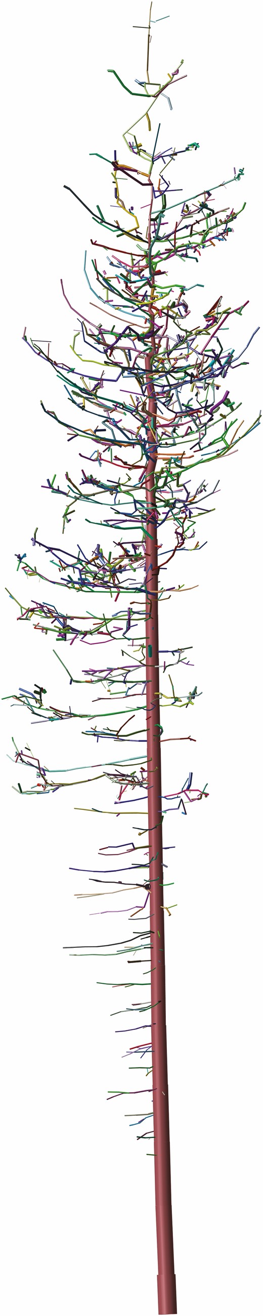
Example of a quantitative structural model (QSM). QSMs are vital for extracting detailed structural measurements of woody plants useful in downstream analysis such as FSPM input or validation and calibration. Cylinders are used to reconstruct 3-D structure from point cloud data. Here, the different colours represent the different branches of the tree.
Differentiating between individual trees remains a key challenge when working with scans containing multiple trees. Whilst this is simple enough to do manually using open-source software such as CloudCompare, it becomes increasingly time-consuming relative to the size of the area covered as well as the density and structural detail of trees. Automated or semi-automated methods can help to streamline this area of TLS data processing (Fig. 5). However, error propagation arising from TLS automated workflows is a known issue and human assistance should be used where appropriate (Martin-Ducup et al., 2021). There are at least two open-source software options available that tackle this issue in different ways. Firstly there is treeseg (Burt et al., 2018) and 3dforest (Trochta et al., 2017), both developed with C++, which use a number of standard point cloud processing techniques; and secondly there is LidR (Roussel et al., 2020), written in the R environment, intended for use with airborne LiDAR, but easily applied to TLS. These software options are invaluable for reducing the amount of time for point cloud processing in forest environments. However, due to the popularity of the R language in biological sciences compared with C++, LidR has the added benefit of accessibility.

Segmentation of individual trees from a whole-forest scan. Although manual segmentation is possible, automation or semi-automation of this process can greatly speed up the processing of TLS data. The different colours delineate between individual trees in the forest community.
Extensive point clouds of multiple trees become even more difficult to handle when they include different materials (i.e. leaf and wood) (Côté et al., 2012). It is often recommended to complete scanning campaigns in leaf-off conditions but there are many scenarios where that may not be possible, or even desired, such as when calculating leaf area index or leaf area distribution. Therefore, a method of separating leaf and wood from point clouds is essential for working with TLS data in an ecological context. Indeed, calculations of leaf area index can be overestimated if woody material in the canopy is unaccounted for (Woodgate et al., 2015). Similarly, woody AGB estimates can be overestimated if leaf points are unaccounted for. Methods for separating leaf and wood fall largely into two groups: geometric-based separation and intensity-based separation. Intensity-based methods use the measured intensity of the laser beam as a marker of the material, using a simple threshold value for the classification. However, this kind of simple approach does not perform well in general. The intensities may still be useful for classification as one of the information sources (X. Zhu et al., 2018). Geometry-based methods compute multiple geometrical features characterizing each point’s neighbourhood and then train a leaf–wood classifier based on those features. With the variety of approaches available it can be daunting to select an appropriate method for a particular study. More recently, a method has been described with a high level of automation as well as options for flexibility. TLSeparation is an open-source Python library offering custom workflows and automated scripts (Vicari et al., 2019). This software performs with a 90 % accuracy for separating leaf and wood in field TLS data, which is a beneficial step towards efficient TLS data processing of large forest scans. There are other geometric-based published methods with similar accuracies (Wang et al., 2018, 2020; Moorthy et al., 2020).
Species identification
An area of TLS research with exceptional benefits to ecological modelling is the development of automatic species identification algorithms. A handful of studies have investigated potential methodologies in different scenarios. Othmani et al. (2013) used bark texture to identify five species from a sample size of 75 individuals using a random forest classification with an accuracy of 85 %. While this method can be useful for identifying species that are mostly different only in their bark, the required accuracy and resolution levels require close-range scanning. Barmpoutis et al. (2018) classified four species of Caatinga trees using the fast-marching method for tree skeletonization, subsequently classifying skeletons with descriptors that account for a combination of dynamic, appearance and noise parameters. Whilst this method outperformed alternative approaches based on geometric characteristics, the sample size (15 individual trees) is too low to determine whether or not it would be feasible to apply this methodology to large forest scans with lots of individuals.
Some success has been found with large sample sizes in studies using QSMs to obtain structural features and machine learning for classification. Åkerblom et al. (2017) obtained an average classification accuracy of >93 % in a single-species forest plot, with lower accuracy found in mixed-species plots. A more recent study by Terryn et al. (2020) expanded on this work using a mixed species plot of 760 trees across a 1.4-ha study area to compare classification. They were able to achieve a classification success rate of 80 %, but with lower accuracies for three out of the five target species. High intraspecific variation alongside low inter-specific variation led to classification complications, which are difficult to overcome in mixed-species plots. The authors find that the greatest factor contributing to classification success is canopy class. Whilst these results are not entirely surprising, they do exemplify the frustrating difficulty in applying quantitative techniques to organisms with high levels of local adaptation. Moreover, Martin-Ducup et al. (2020) found a convergence of tree architecture with increasingly dominant crown canopy positions in tropical trees. They interpreted this convergence as resulting from a liberation effect of canopy trees from side-shading constraints. These results also point to the challenges of using structural metrics for species identification. Further research is required in this area as FSPMs require species-specific information to function reliably, and any ability to automatically identify species across large areas would greatly improve the potential to apply FSPMs to larger ecological questions.
TLS in studies of vegetation dynamics
TLS data, often with derived QSMs, have been used to gain new understanding of forest dynamics and structure. For example, Seidel et al. (2011) showed how crown plasticity in terms of crown asymmetry is used by trees to avoid competition. They concluded that TLS offers an opportunity to achieve a better understanding of the dynamics of canopy space exploration, which can produce valuable advice for the silvicultural management of mixed stands. Kunz et al. (2019) studied the crown plasticity more thoroughly by scanning thousands of trees in large-scale forest experiment plots with variable species mixtures with TLS. They found that crown complementarity and crown plasticity increased with species richness. Furthermore, trees growing in more species-rich neighbourhoods showed enhanced above-ground wood volume in trunks and branches, and over time the diversity induced shifts in wood volume allocation in favour of branches. Martin-Ducup et al. (2018), in turn, found that the foliage distribution of sugar maple shifted towards the crown base in mixed stands when compared with pure stands. Recently, van der Zee et al. (2021) introduced a novel method of quantifying the phenomenon of ‘crown-shyness’ by applying a 3-D surface complementarity metric to TLS data. With this method they were able to exemplify local adaptive responses in neighbouring trees and the relationship between crown complementarity and individual ‘slenderness’ mirroring previous results. Applying TLS in a functional context, Hildebrand et al. (2021) found no support that functional dissimilarity promoted crown complementarity in a mixed-species forest stand. Rather, they find that the relative efficiency of different species in occupying canopy space is better explained by phenotypic changes related to crown morphology and branch plasticity. This has interesting implications for how we view woody plant interactions, highlighting the need for a thorough 3-D approach to forest community ecology.
The phyllotactic patterns of many herbaceous plants are generated by a constant divergence angle between successive buds that first appears at the shoot. Beyer et al. (2021) investigated whether the branches along tree trunks exhibit a similar constant divergence angle. From branch skeleton data derived from TLS data they empirically estimated the distributions of the divergence angles between successive branches along the trunks. They found that, rather than having species-specific branch divergence angles, mature European beech, Norway spruce and Scots pine trees feature statistical properties characteristic of a uniform distribution. They hypothesized this to be the result of the stochasticity in bud development and branch shedding, and showed that the distribution of branch divergence angles will approximate a uniform distribution if bud mortality and branch shedding rates are high.
Calders et al. (2015b) monitored the timing of recurring seasonal dynamics through the plant area index (PAI). From TLS data they estimated vertical plant profiles, which describe the plant area per unit volume as a function of height. They generated a time series from 48 measurement days in a deciduous forest and the start of season was observed to depend on the species composition. They concluded that phenological differences will be more pronounced in multi-layered forests, and TLS was shown to have the potential to study seasonal dynamics not only as a function of time, but also as a function of canopy height. An exciting advancement in the area of TLS time series for monitoring forest dynamics is described by Campos et al. (2021), where they outline the creation of an automated and permanent TLS measurement station. This new monitoring station is the first to collect long-term TLS data at 1-h intervals. In preliminary results they were able to identify a number of short-term and long-term changes in a boreal forest, notably the short-term circadian rhythms in silver birch trees over 30 h, and longer-term phenological chances of spring leaf-sprout and stem diameter growth.
A number of studies have used TLS to investigate relationships between environmental factors and woody plant structure. TLS data and the derived QSMs of trees have been used for mechanical modelling of the trees under critical wind speeds (Jackson et al., 2019). Mechanical stability is a vital component of woody plant form and function and here it was found that the difference in critical wind speed is driven by tree size and architecture, rather than material properties. In this study a trade-off between critical wind speeds and growth rate was also observed. Van der Zande et al. (2010) combined TLS measurements with a voxel-based light interception model to examine the relationship between variable light conditions and the distribution of leaves in 3-D space; their results exemplify the impact of neighbourhood crown size on the available light in the canopy.
Using TLS to parameterize FSPMs
Once the individual trees are isolated from the TLS point cloud, and the points from leaves are removed if necessary, it is possible to calculate many useful structural metrics. Straightforward calculations are available for macroscopic metrics, such as height, crown diameter and convex bounding volumes. But more specific metrics, such as diameter at breast height, stem volume, crown ratio and branch lengths and volumes, require more processing, often some kind of segmentation of the point cloud into suitable tree parts. An effective way of reconstructing the whole woody structure is through the implementation of QSMs. The use of QSMs generates possibilities to use TLS data for FSPMs (Fig. 6). Firstly, simulating physiology and environment in a static context can directly use empirical tree models derived from TLS data. Secondly, these empirical structure models are useful for providing data needed to validate and test the 3-D structure of FSPMs against empirical data in order to estimate their accuracy and usefulness more generally. For example, measuring detailed and complete structural information, such as branching topology and diameters, of large trees with manual measurements is very laborious or even practically impossible. With TLS it is possible to quickly collect such data from a large number of individuals that form a representative sample. This often requires that the TLS data are first transformed into QSMs, from which the structural tree data can be computed and inferred. However, much of the required structural information can be estimated from TLS data without full QSMs, namely overall measures such as crown dimensions and woody plant height. Moreover, useful information about the leaves, such as total leaf area (Béland et al., 2011) and leaf orientation (Zheng and Moskal, 2012) together with their spatial distributions, can be estimated from TLS data. Thirdly, the non-destructiveness of TLS allows for repeated measurements over a span of time, for example over a growth season or many years. This way it is possible to produce an empirical time series of 3-D architecture and sample growth dynamics. These time series can similarly be used to validate and test the accuracy of the dynamic modelling of woody plant growth in a given FSPM. Lastly, time series data are useful for initialization, calibration or optimization of the FSPM parameters to make them correspond better to the observed form and function of woody plants.
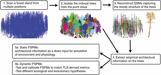
A potential TLS to FSPM workflow. 1. To minimise occlusion and gain an even point coverage, individuals should be scanned from multiple positions at regular intervals (see Wilkes et al. 2017). 2. Trees can be segmented from the large scan using segmentation software, LidR (Roussel et al. 2020) treeseg (Burt et al. 2018) or 3DForest (Trochta et al., 2017). 3. Generate QSMs for each individual in the scan (Raumonen et al. 2013) 4. Extract the appropriate structural information for use in FSPMs. 5a. Structural information can be used directly to simulate function with static woody structure and changing environmental conditions. 5B. Alternatively, structural information can be used to initialise FSPMs, aid validation and calibrate dynamic models with changes in woody structure.
A concrete example of using TLS data for parameterization and validation of FSPMs, at a proof-of-concept level, was given by Sievänen et al. (2018). In this study, pine trees of different ages but in the same location were scanned with TLS. This created a pseudo-time series of growth of a single tree. From the TLS data, empirical cylindrical QSMs were reconstructed to model the tree architecture at each age interval of the tree. To complete the models with needle information, the location of needles was also estimated from the TLS data and together with needle allometry their area was estimated. The empirical tree models were thus similar in form as in LIGNUM. Then within the LIGNUM model many different crown development mechanisms were formulated and their parameters were optimized so that the resulting models matched as closely as possible many architectural attributes of the corresponding empirical tree models. The hypothesized mechanisms that most closely matched the empirical tree models were then considered more likely to capture the details of real crown development mechanisms. TLS data and QSMs were similarly used by Potapov et al. (2016), where they proposed a stochastic version of LIGNUM for producing tree structures consistent with detailed TLS data. They did the matching by iteratively finding the best correspondence between the empirical QSMs and the stochastic choices of the algorithm. They concluded that the proposed approach is a viable solution for realistic plant models based on data and accounting for the stochastic influences. The trees produced with their data-based model resemble the real measured trees and are statistically similar but not copies of each other. Later they expanded the idea to general stochastic structure models and showed how to generate data-based morphological tree structure clones (Potapov et al., 2017).
Figure 6 specifies the principal steps in the TLS to FSPM workflow for simulation of tree communities. Although this paper has shown examples of these steps, there are still many obstacles that have to be overcome in order for the workflow to be an easy one to apply. For example, in step 1, when scanning a forest from multiple positions, there comes a point when the density of woody plants is too great to allow for efficient placement of TLS instruments. This in turn results in high occlusion of woody branches or missing areas entirely if it is not possible to reach all areas of a survey site. One way of overcoming this issue is by using LiDAR-mounted unmanned aerial vehicles (UAVs) to complement ground-based TLS in order to minimize data gaps (Brede et al., 2019; Schneider et al., 2019). Density of woody plants in a forest stand can also greatly impact step 2. if there is significant branch overlap between neighbouring plants, automated and semi-automated methods may struggle to distinguish which branches belong to which plant. Species can also impact individual isolation from a point cloud if there are many species with a low, shrubby growth habit. Many of the separation algorithms rely on the ability to identify a distinct trunk close to the ground, and if this is not possible manual isolation may be required.
After step 2 the challenge of step 3 and its applications for FSPMs is acquiring botanically accuracy in QSM reconstruction. The way QSMs are reconstructed usually cannot produce a botanically faithful architectural structure. For example, it may be that e.g. internodes are not correctly identified or foliage (if it is detected) is placed in internodes that botanically cannot carry it. For some species and with good enough quality data, it is possible to post-process QSMs to proper botanic form. However, for example if dead branches are broken off the stem, this may not leave any discernible trace in the TLS data and thus it is impossible, at least reliably, to reconstruct botanically correct QSMs. Following this, step 4, deriving architectural metrics, is just one part of FSPM parameterization. In this step, in addition to architectural structure, FSPMs require data for environmental and physiological sub-models. Such data are not available from TLS measurements, except for optical properties of foliage and woody parts. These data can be obtained from other models, flux towers or trait databases or existing literature. Differences between parameter requirements of different of FSPMs will dictate the difficulty of finding these values. In addition, the parameter values vary with growing conditions, e.g. site quality. Therefore, if the TLS scan does not provide information on foliage, the foliage must be generated using additional information contained in parameter values or calculated (Lintunen et al., 2011). If a TLS scan is used to initialize forest structure for a simulation, then also the initial values of all variables in a FSPMs dynamical equations are required (i.e. amount of sapwood). This is best accomplished using a special module of the FSPM that calculates initial values as a function of the architectural structure and parameter values. Lastly, a botanically correct architectural structure, including positions of buds that flush to produce growth (Fig. 2), is preferable for starting of simulation.
DISCUSSION
TLS has already transformed the way we collect data on forest communities, providing unparalleled information about the spatial arrangement of individuals and their interactions in 3-D space, yet currently largely limited to the detection of static and transient patterns between the diversity of vegetation structure and other community features (Davies and Asner, 2014; D’Urban Jackson et al., 2020). FSPMs are capable of scaling structural relationships between different organs of the same plant to the structural relationships of whole plants in the same community. Using TLS together with FSPMs, in turn, forms a promising toolkit to explore questions involving longer time spans in forest community ecology and evolution. The availability of structural data for a wide range of species, across a wide range of habitats is key for shifting the focus of FSPMs from a practical use to a more paradigmatic one. Indeed, TLS data are already available for forest communities in numerous databases (Guzmán et al., 2020), with more data being collected and openly shared over time. Both TLS and FSPMs are associated with large amounts of data and parameters and high computational demand; however, no other combined method is capable of capturing, testing and investigating the spatiotemporal dynamics of forest communities in such detail. When used in tandem, FSPMs and TLS could be used to test hypotheses for dynamic relationships between biodiversity and productivity, ecosystem functioning and resilience to species losses or invasions in forest communities. Whilst these questions have been explored through several experimental studies, the studies that cover all phases of structural development of existing vegetation have exclusively been carried out with herbaceous plants and so have a limited applicability for forest ecosystems (Naeem et al., 1994; Tilman and Downing, 1994). Several experimental studies of tree diversity have been established but even the oldest ones cover only ~20 years of forest development (https://treedivnet.ugent.be). Time is a difficult barrier to overcome in experimental studies of forest structure and dynamics. Whilst sudden changes in a forest community such as tree fall are easily detectable, long-term patterns may take decades to emerge. Using TLS and FSPMs together to generate models of forest development maintains a high level of structural realism and overcomes the limiting factor of time by simulating changing environmental conditions. The potential of this synergy is exciting but there are still a number of challenges that need to be overcome before it can reach its full potential.
In a recent review of agent-based models in plant science and ecology, Zhang and DeAngelis (2020) state that although FSPMs are set up in such a way that they should be able to address many of the same questions as population-level agent-based models, it is not yet possible to apply FSPMs at the landscape level. It may not be even desirable to use FSPMs at that level. However, scaling up from organ to tree community level is necessary and interesting for problems of forest community ecology and evolution. There are only a few applications of FSPMs that simulate tree communities as interacting individuals and this facet of FSPM research is not yet well developed. However, several of the models in Table 1 are able to cope with multitree simulation. The examples for computing environment requirements in the General features of FSPMs section show that FSPMs are able to simulate stand level forest communities with is no principal impediment to using them in such studies. Available computer resources are not an obstacle to simulating a sizable tree community either.
In order to increase the utility of FSPMs in ecology and evolution of forest communities, the focus of development must shift towards a more general approach. Firstly, physiological processes must be easily parameterized. There are numerous ways of modelling basic physiological processes, and it would be beneficial to be able to parameterize the physiological sub-model depending on the context of the study. The FSPMs of Table 1 have been parameterized for several tree species. The parameterizations are nevertheless very model-specific: using the parameter values in another model requires tedious handwork. If this problem could be alleviated, for example through a parameter database as a part of model website (www.quantitative-plant.org), it would speed up applying FSPMs. Secondly, it is essential to have flexibility with regard to the architectural sub-model. For FSPMs to be broadly applied in the ecology and evolution of woody plants it is imperative that a range of structural forms are easily defined. Of the 21 different architectural forms described by Hallé and Oldemann, only a handful have been featured in published FSPMs (Hallé et al., 1978). However, to exchange architectural sub-models, FSPMs could be better suited to deal with input parameter values. Many models apply a formalism [L-systems (Lindenmayer and Prusinkiewicz, 1990) in the first place] to deal with morphological development. This opens possibilities of automatic transfer and translation of architectural information. Further, there exists a formalism to code architectural information, the multiscale tree graph (MTG, Godin and Caraglio, 1998), that can be used to transfer architectural information between FSPMs (Boudon et al., 2012). Lastly, increasing the use of TLS-derived data is one way of overcoming the lack of structural forms found currently in FSPMs; however, only one published FSPM, HELIOS, features open-source TLS integration software (Bailey, 2019). For FSPMs to be readily scaled up to the population level, a dedicated TLS pipeline must become an integral part of FSPM development.
The sampling design proposed by Wilkes et al. (2017) for TLS studies could serve as a reasonable baseline for simulating community-level FSPMs. As interest in using TLS for characterizing forest structure grows, so will the availability of TLS datasets. If TLS could be used to rapidly assess forest plots across a landscape, this could be used to inform multiple FSPM simulations across a larger geographical area. Moreover, repeated scans of the same area can provide invaluable temporal data, important to understanding phenology and sensitive responses over time highlighted by Campos et al. (2021). The quality and quantity of structural data provided by TLS give FSPM developers the opportunity to make better decisions about the detail and scale of their models, as they are no longer being constrained by the specific set of parameters available. Data captured by TLS automatically covers several levels of structural detail with nearly the same sampling effort. Thus, the data captured by TLS enable the researcher to flexibly make choices about the level of detail employed for research and also to use the data and models to iteratively check how the ecological or evolutionary predictions depend on the level of detail utilized.
In Fig. 6 we describe a potential TLS to FSPM workflow, starting with a forest point cloud and ending with either architectural input for FSPMs or validation and calibration. At each step of the workflow there are multiple software options available and a crucial step in expanding its uptake is a better understanding of the differences between these software options. Benchmarking and comparison have long been a shortcoming of FSPM development, as noted in several reviews (Louarn and Song, 2020; Zhang and DeAngelis, 2020). Indeed, model complexity, inconsistency between sub-model representation, varied input parameters and a lack of open-source code has hindered a thorough evaluation of models (Table 1). However, a few groups have endeavoured to improve this situation, notably in the area of below-ground FSPM development. Schnepf et al. (2020) issued a call for participation for a collaborative effort to compare root FSPMs via a two-step system, firstly by identifying a number of ‘benchmarking scenarios’ and secondly by coupling these scenarios with specific research questions. This incremental method can therefore identify differences arising in step 1 which could impact step 2 in ways that would otherwise go unnoticed. Above-ground FSPMs could greatly benefit from a similar approach, and it will be important in upcoming years to improve communication between groups to tackle this issue.
From a TLS perspective, it is also important to ascertain areas of potential divergence in the workflow such as those related to the instrument used or QSM generation. To date, no formal comparison of TLS instruments exists, and it is possible for different instruments to return different results for the same target (Orwig et al., 2018). Scanning from multiple positions, as suggested in Fig. 4, will reduce bias, but, depending on the terrain and equipment, could significantly increase the scanning time. Furthermore, there are limits to how well TLS instruments can capture fine branches and leaves in real field scenarios where even slight wind could introduce substantial noise. Any errors accumulated during the scanning process will only be exacerbated in downstream automatic and semi-automatic methods (Martin-Ducup et al., 2021). For example, low point densities may produce inaccurate QSMs, and without a manual method of validation it is unclear how this might impact architectural input parameters for FSPMs (Disney et al., 2019). Care must also be taken regarding woody plants that do not have a typical ‘tree-like’ structure. Most of the software available for individual segmentation and QSM construction assume that individuals have a singular trunk. However, forests globally contain a variety of forms and it is important that methods can be applied with equal accuracy across all architectural types. Furthermore, most TLS studies have been conducted in temperate, boreal or tropical forest, with little representation in dry forest or savannahs, where woody plants tend to have a more shrub-like growth habit (Muumbe et al., 2021).
A key difference between using FSPMs in horticulture and agronomy and FSPMs in ecology and evolution is that development will ultimately be driven by the search for emergent patterns. FSPMs have long been designed based on the research question at hand, usually for a specific species or outcome. This has made it relatively straightforward to select appropriate sub-models depending on the context. However, designing FSPMs to represent emergent patterns of forest structure and dynamics will require a thorough evaluation of the sub-models included. Evers et al. (2019) suggested guidelines for creating mixed-species FSPMs, noting that any neighbourhood interactions should emerge only as a result of individuals requiring and acquiring resources in a given community, and not as an explicit process in the model. The use of mixed-species FSPMs is a relatively recent direction of research but the empirical observations from TLS studies of vegetation dynamics can hopefully guide model development.
OUTLOOK AND CONCLUSIONS
Since the emergence of FSPMs over two decades ago, there has been an explosion of research into many different facets of this modelling paradigm, with many successes in agronomy and horticulture. Despite this, applications of FSPMs to forest community ecology and evolution have not proceeded at the same pace. We believe that FSPMs, in combination with TLS-derived data, can finally begin to address ecological and evolutionary dynamics in forests. For the potential of this synergy to be realized, a number of challenges need to be addressed. First, FSPM research already spans many disciplines, including life sciences, computer science and mathematics. However, effectively using FSPMs for forest communities requires coordination between plant ecophysiologists, ecologists and evolutionary biologists. This will be essential for linking detailed organ-level processes with community-level processes to improve the explanatory power of FSPMs. Second, efforts must be made to enhance the generality of FSPMs. TLS-derived data have expanded the structural generality of FSPMs immensely, but general methods of implementing the physiological and environmental sub-models still require attention. One way of improving this is to encourage FSPM developers to produce open-source code and participate in benchmarking efforts. Third, TLS data have largely been collected for ‘tree-like’ plants. For a comprehensive understanding of woody plant form, TLS campaigns need to take place in a variety of forest environments, including tropical dry forests. Both FSPMs and the use of TLS for forest surveying are still in their early days but there is a great deal of potential when these tools are combined. The ability to simulate realistic structure and dynamics in forest communities with FSPMs fulfils a specific niche in the spectrum of vegetation modelling. Phenomena that eventually contribute to regional and ecosystem structural diversity and vegetation patterns ultimately occur on a local scale, and thus it is essential not to neglect the impact of fine-scale changes in forest communities.
FUNDING
This work was supported by the National Environment Research Council (grant number NE/P012345/1) and the Academy of Finland (‘Centre of Excellence of Inverse Modelling and Imaging’ project).
ACKNOWLEDGEMENTS
We thank Iain Colin Prentice, Justin Moat and James Rosindell for comments on the manuscript.
