


Abstract
The geographical distribution of plant species is linked fundamentally not only to environmental variables, but also to key traits that affect the dispersal, establishment and evolutionary potential of a species. One of the key plant traits that can be expected to affect standing genetic variation, speed of adaptation and the capacity to colonize and establish in new habitats, and therefore niche breadth and range size, is the plant mating system. However, the precise role of the mating system in shaping range size and niche breadth of plant species remains unclear, and different studies have provided contrasting results. In this study, we tested the hypothesis that range size and niche breadth differed with mating system in the orchid genus Epipactis.
We modelled the ecological niches of 14 Epipactis species in Europe using occurrence records and environmental satellite data in Maxent. Niche breadth and niche overlap in both geographic and environmental space were calculated from the resulting habitat suitability maps using ENMTools, and geographic range was estimated using α-hull range definition. Habitat suitability, environmental variable contributions and niche metrics were compared among species with different mating systems.
We did not detect significant differences in niche breadth, occurrence probability or geographical range between autogamous and allogamous Epipactis species, although autogamous species demonstrated notably low variation in niche parameters. We also found no significant differences in niche overlap between species with the same mating system or different mating systems. For all Epipactis species, occurrence was strongly associated with land cover, particularly broad-leafed and coniferous forests, and with limestone bedrock.
These results suggest that the mating system does not necessarily contribute to niche breadth and differentiation, and that other factors (e.g. mycorrhizal specificity) may be more important drivers of range size and niche breadth in Epipactis and orchids in general.
INTRODUCTION
Understanding the various factors that determine the geographic distribution and niche breadth of plant and animal species is one of the key topics in ecology and evolutionary biology (Brown et al., 1996; Sexton et al., 2017). Niche breadth, or the range of habitat conditions encompassed by a species’ ecological niche, is defined as the distance between the mean habitat conditions of a species and the mean habitat conditions across the study area (Dolédec et al., 2000). Habitat generalists tolerate a wide range of environmental conditions, or have broad niches, in comparison with habitat specialists, which have narrow niches and inhabit a smaller array of environments. In general, the range size and niche breadth of a species are limited by traits that affect its dispersal, population dynamics and evolutionary potential (Gaston, 2003). Species that possess traits that facilitate dispersal and colonization of new habitats or that have high genetic variation, and hence high evolutionary potential, can be expected to have larger distribution ranges and wider niche breadths than species that lack these traits. Because species within a single genus may strongly differ in key plant traits, the range sizes and niche breadths of even closely related species can differ substantially (Brown et al., 1996; Grossenbacher and Whittall, 2011; Anacker and Strauss, 2014).
One of the traits that can be expected to have a large impact on range size and niche breadth is the plant mating system (Geber, 2008; Randle et al., 2009; Petanidou et al., 2012; Grossenbacher et al., 2015; Grant and Kalisz, 2020). Because selfing species tend to have lower standing genetic variation than outcrossing species (Hamrick and Godt, 1996; Honnay and Jacquemyn, 2007), this may restrict their ability to adapt to changing environmental conditions (Fisher, 1958; Holt and Gaines, 1992) and therefore decrease their distribution ranges and niche breadths. The transition from allogamy to autogamy has been considered to be an evolutionary dead-end because of selfers’ inability to adapt to new environments as a result of inbreeding depression (Stebbins, 1957; Takebayashi and Morrell, 2001; Gamisch et al., 2015). On the other hand, unlike outcrossing species, selfing species do not rely on the availability of pollinators and compatible mates to reproduce in a new environment, and may therefore be able to expand their ranges more easily (Baker, 1955). Additionally, the gene flow caused by outcrossing can limit the concentration of certain alleles that lead to the evolution of adaptive traits (Levin, 2010; Paul et al., 2011), resulting in outcrossing species being less well equipped to adapt to new environments and consequently having narrower niche breadths and smaller ranges than autogamous species (Grossenbacher et al., 2015). Because selfing acts as a reproductive isolation barrier (Brys et al., 2016, 2014), it will limit the influx of maladaptive genes and may increase the rate of adaptive evolution (Levin, 2010), and thus increase niche expansion.
At present, few studies have investigated the relationship between the plant mating system and niche breadth, and these studies have revealed contrasting results. For example, Grant and Kalisz (2020) recently showed that selfing species had significantly wider niche breadths than outcrossing species. Similarly, Randle et al. (2009) and Grossenbacher et al. (2015) showed that selfing species had larger distribution ranges than outcrossing species. In contrast, a study conducted by Park et al. (2018) of >400 species indicated that mating system was not a strong predictor of niche breadth for plant species. Similarly, Johnson et al. (2014) showed that although the geographic ranges of selfing Fragaria species were larger than those of outcrossing species, there was no effect of mating system on ecological niche breadth. Given these contrasting predictions, it is not entirely clear how the mating system affects the distribution and niche breadth of plant species, and is likely to be variable among taxa.
In the Orchidaceae, selfing is relatively common compared with other plant families, with 31 % of species able to self-pollinate (Peter, 2009), but its influence on distribution and niche breadth remains unclear. Despite the large number of seeds produced by orchids and their high dispersal potential (Arditti and Ghani, 2000), most orchid populations tend to be small and isolated (Otero and Flanagan, 2006), suggesting that their distributions must be limited by factors other than dispersal ability (McCormick and Jacquemyn, 2014). The distribution of orchids, as with other plants, is influenced by a combination of biotic and abiotic factors that determine successful fertilization and seed production, seed dispersal and germination, seedling establishment and survival to adulthood. Fruit set in orchids is generally low (Tremblay et al., 2005), and the evolution to selfing clearly provides reproductive assurance and allows orchids to reproduce in habitats where pollinators are scant or lacking (Brys and Jacquemyn, 2016) and therefore may allow rapid colonization of novel habitats and increased niche breadth. Evolution to selfing also represents an important barrier to gene flow and may facilitate genetic and morphological divergence between taxa, ultimately leading to speciation. However, the extent to which variation in the mating system affects the distribution range and niche breadth of orchids remains unknown.
In this study, we used ecological niche modelling to investigate the distributions of Epipactis species in Europe and to compare the components that define their ecological niches. The genus Epipactis contains a complex of allogamous and autogamous species, among which species limits are not always easy to define (Hollingsworth et al., 2006; Sramkó et al., 2019). Moreover, Epipactis species display wide variation in geographic distribution (Ehlers and Pedersen, 2000; Efimov, 2008) and therefore represent an ideal study system in which to study the effects of mating system variation on distribution range and niche breadth. Mating system transitions and changes in pollination strategy that allow establishment and survival of newly colonized habitats have been invoked to explain the diversification of the genus (Hollingsworth et al., 2006; Tranchida-Lombardo et al., 2011). However, little is known about how the mating system affects range size and niche breadth. Specifically, we tested the hypothesis that autogamous species have broader niches than allogamous species by comparing niche breadth and range size between species with different mating systems. The results of these investigations may shed light on the contribution of the mating system to the divergence of a taxonomically complex genus through differential adaptation to abiotic environmental components.
MATERIALS AND METHODS
Study species
Fifteen Epipactis (Orchidaceae) species were selected for analyses based on having at least 30 occurrence records available. Due to the taxonomically complex nature of the genus Epipactis and the difficulties that arise as a result of the existence of morphologically distinct ecotypes, multiple names probably exist for the same species; indeed, Bateman, 2020 considers there to be no legitimate Epipactis species at the local level. To reduce the likelihood of analysing a single species under two names, we used the recent phylogeny of the genus created by Sramkó et al. (2019) to choose ten species that are distinct enough from one another to be considered species with sufficient certainty: E. albensis, E. atrorubens, E. dunensis, E. helleborine, E. leptochila, E. lusitanica, E. muelleri, E. palustris, E. phyllanthes and E. purpurata. Additionally, Sramkó et al. (2019) indicated that E. rhodanensis and E. bugacensis fall under E. dunensis and so we analysed the location records of E. rhodanensis and E. bugacensis as part of E. dunensis. Epipactis microphylla and E. tremolsii were also included because there is strong support for their being monophyletic species in phylogenetic and morphometric research (Bernardos et al., 2004; Hollingsworth et al., 2006; Zhou and Jin, 2018). The species status of E. kleinii and E. fageticola has yet to be tested with genomic analyses; however, we include these here as E. kleinii, a new name for E. parviflora, is considered to be distinct by Crespo et al. (2001), and morphological and ecological analyses suggest that E. fageticola is probably also a species (Gévaudan et al., 2001). Included are species that are very localized, such as E. tremolsii which has been recorded only in the western Mediterranean area (Bernardos et al., 2004), as well as widespread species, such as E. helleborine which can be found from western Europe to China (Xing et al., 2020).
Occurrence data
Records of each species’ occurrence from 2000 to 2020 for the continent of Europe were obtained from the online database GBIF (www.GBIF.org). We discarded records with missing GIS co-ordinates, ambiguous species identification or with co-ordinates with a spatial resolution lower than approx. 100 m (three decimal places). The number of resulting species records varied between 31 (E. lusitanica) and 45 354 (E. helleborine), with the majority of species having >100 records (Supplementary data File S1). Records for each species were spatially filtered by aggregating records in 10 km2 grid cells and extracting the centre co-ordinates of each grid cell in which the species was recorded, to reduce the effects of spatial clustering resulting from sampling bias (Boria et al., 2014). Processing of occurrence data was performed in QGIS v3.4.9 (QGIS Development Team, 2019).
Ecogeographic variables
The ecological niche of orchids has been shown to be a function of precipitation and temperature, altitude, soil composition, bedrock and vegetation type. We therefore used a total of nine raster-format predictor variables with <0.5 correlation with one other. Two of the 19 bioclimatic variables available from the WorldClim online database (Hijmans et al., 2005) (http://worldclim.org/version1) were chosen for use in our model, i.e. mean annual temperature and annual precipitation. Two topsoil datasets were acquired through the European Soil Data Centre (ESDAC), one consisting of six physical measurements of soil texture and water availability (Hiederer, 2013; https://esdac.jrc.ec.europa.eu/content/european-soil-database-derived-data) and the other consisting of six biochemical levels and pH (Ballabio et al., 2019; https://ec.europa.eu/eurostat/web/lucas/data/primary-data/2018). A principal component analysis (PCA) was performed on both sets of variables, and the rasters of the first two axes were used as predictors. Two categorical variables were acquired: dominant bedrock from the ESDAC database (Van Liedekerke et al., 2006); https://esdac.jrc.ec.europa.eu/resource-type/european-soil-database-maps) and Corine Land Cover (CLC) from the Copernicus program of the European Environmental Program (Heymann, 1994; https://land.copernicus.eu/pan-european/corine-land-cover/clc2018). An elevation raster was also included as a predictor variable (Amatulli et al., 2018; https://www.earthenv.org/topography). All rasters had a spatial resolution of 1 km, except for land cover, which had a resolution of 100 m and was resampled to match the resolution of the other rasters. Raster processing was performed in RStudio v3.6.2 (R Core Team, 2019) using the ‘raster’ (Hijmans et al., 2005) and ‘RStoolbox’ (Leutner et al., 2017) packages.
Ecological niche modelling
We used the program Maxent v3.4.1 (Phillips et al., 2017) to create ecological niche models for the 15 Epipactis species. Maxent uses species occurrence data and environmental rasters to calculate a Gibb’s P-value for each pixel of the study area, representing the probability that the pixel has suitable conditions for the species (Phillips, 2005). Maxent then creates habitat suitability maps by projecting the ecological niche model onto the geographic space of the study area. In addition to these maps, Maxent produces a table of the percentage contribution of each predictor variable to the distribution of suitable habitat of each species. The choice of Maxent settings was informed by Barbet-Massin et al. (2012) and Merow et al. (2013). Each model was run using a random seed, and 100 bootstrap replicates with 75 % of the data were used to train the model and 25 % to test it. The variables ‘land-use’ and ‘bedrock’ were specified as categorical variables through the Maxent GUI (see Merow et al., 2013 for more details on how Maxent handles categorical variables). The rest of the settings were left as the default (convergence threshold of 0.00001, regularization threshold of 1 and a maximum of 10 000 background points) and allowed for linear, quadratic, product and hinge features to be chosen automatically, producing a cloglog output. Model performance was assessed using AUC (area under the receiver–operator curve), with values closer to 1 indicating good fit.
A cluster analysis was performed on the Maxent output table of variable contributions to investigate whether species could be grouped based on similarity in habitat preference. Five agglomerative clustering methods were performed on a Euclidean distance matrix of the data, and the best method was chosen based on having the smallest cophenetic correlation value. The number of clusters to use was assessed using the silhouette width and Mantel approaches. The contribution of each variable to the species’ estimated distribution maps was then plotted as a heat map. These analyses were performed in RStudio v3.6.2 (R Core Team, 2019) using the ‘cluster’ (Maechler et al., 2012), ‘gclus’ (Hurley and Hurley, 2019) and ‘pheatmap’ (Kolde and Kolde, 2015) packages.
Geographical range
The area of each species’ current spatial range in Europe (unlike the projected distribution based on environmental variables described above) was determined by creating an α-hull polygon around each species’ occurrence points (Edelsbrunner et al., 1983; Burgman and Fox, 2003). This was done by performing Delaunay triangulation on a species’ locality points, calculating the mean line length and multiplying it by an α value of 5, and removing any lines longer than this number. This was performed using the ‘alphahull’ package (Rodríguez Casal and Pateiro López, 2010) in RStudio v3.6.2 (R Core Team, 2019). The resulting polygons were then exported to QGIS v3.4.9 (QGIS Development Team, 2019), clipped to the boundary of Europe to exclude oceans and seas from the distributions, and the areas extracted for each species. GBIF data mainly consist of records resulting from random field sampling and sampling restricted to certain areas, and so are unlikely to encompass the entire geographic ranges of species. For example, E. albensis is only evident in France in our data but has been recorded by Molnár and Sramkó (2012) in Romania. Therefore, we stress that these α-hull areas are conservative, and are used here purely as European range estimates and for use in comparisons among species.
Niche breadth and niche overlap
The niche breadth in geographical space was calculated for each species as the mean Levins’ B value (Levins, 1968) from 30 replicate habitat suitability maps of each species with the software ENMTools v1.3 (Warren et al., 2010). The ENMTools package was further used to calculate Schoener’s D value in environmental space, representing niche overlap, or similarity in habitat requirements (Schoener, 1968; Warren et al., 2008), for each species pair. We also calculated niche breadth (B2 value) and overlap in environmental space for each species using the ENMTools R package (v 0.2) (Warren et al., 2017). B2 represents the specificity in environmental conditions of a species’ habitat, in comparison with the specificity of the geographic distribution of the potential niche resulting from these ecological associations represented by Levins’ B values (see Peterson et al., 2011 for details on environmental and geographic space). Levins’ B and Schoener’s D values range from 0 to 1, with values closer to 0 representing narrow niche breadth and a small degree of niche overlap, and values closer to 1 representing wide niche breadth and a high degree of niche overlap, respectively. Niche overlap among species was visualized with a correspondence analysis plot using the ‘ca’ package (Nenadic and Greenacre, 2007) in RStudio v3.6.2 (R Core Team, 2019).
Statistical analysis
Mean distribution area, Gibb’s P-value (habitat suitability), variable contributions, Levins’ B value (niche breadth in geographic space), the B2 value (niche breadth in environmental space) and Schoener’s D value (niche overlap) were compared among species with different mating systems and among species clusters using Kruskal–Wallis and Dunn tests with a Holm correction, or analysis of variance (ANOVA) and Tukey tests if the data were normally distributed. We further tested the relationships between mean niche breadth, habitat suitability and geographical range using linear regression performed on log-transformed data. All statistical analyses were performed in RStudio v3.6.2 (R Core Team, 2019).
RESULTS
The AUC values of the Maxent models were >0.8 for all species except E. helleborine, which had an AUC of 0.74. The mean habitat suitability (Gibb’s P-value) predicted by the Maxent model ranged from 0.002 ± 0.007 (s.d.) for E. lusitanica to 0.34 ± 0.253 for E. helleborine (Table 1; Fig. 1), with an average of 0.072 ± 0.028 (s.e.). The areas of the α-hull distributions varied greatly between species, with values between 0.54 (E. albensis) and 938.877 (E. helleborine) decimal degrees (dd) (Table 1; Fig. 1) and a mean area of 223.347 ± 84.557 dd. Levins’ B values (niche breadth) ranged from 0.047 ± 0.004 (E. lusitanica) to 0.642 ± 0.001 (E. helleborine) (Table 1), with a mean of 0.240 ± 0.045 for all the species. Mean Gibb’s P-values (habitat suitability) and Levins’ B values were moderately correlated (R2 = 0.66, P < 0.001). Mean geographical range increased with Levins’ B (R2 = 0.63, P < 0.001) and Gibb’s P-values (R2 = 0.721, P < 0.001). Mean Gibb’s P-values and Levins’ B were not correlated with B2 (niche breadth in environmental space) (R2 = –0.055, P = 0.584 and R2 = –0.055, P = 0.113, respectively) and mean geographical range had a weak positive association with B2 (R2 = 0.178, P = 0.003).
Distribution and niche metrics for each Epipactis species
| Species | Range size (decimal degrees) | Mean Gibb’s P-value (s.d.) | Levins’ B (s.e.) | B2 (s.e.) | Mating system | ||
|---|---|---|---|---|---|---|---|
| E. albensis | 0.544 | 0.006 | (0.0099) | 0.219 | (0.0592) | 0.957 (0.00016) | Autogamy |
| E. atrorubens | 707.340 | 0.207 | (0.2199) | 0.467 | (0.0022) | 0.662 (0.00011) | Allogamy |
| E. dunensis | 37.768 | 0.007 | (0.0125) | 0.223 | (0.0080) | 0.710 (0.00016) | F. autogamy |
| E. fageticola | 5.692 | 0.003 | (0.0060) | 0.186 | (0.0115) | 0.660 (0.00015) | Allogamy |
| E. helleborine | 938.877 | 0.340 | (0.2534) | 0.642 | (0.0010) | 0.643 (0.00026) | Allogamy |
| E. kleinii | 23.300 | 0.003 | (0.0069) | 0.138 | (0.0077) | 0.532 (0.00014) | Allogamy |
| E. leptochila | 115.518 | 0.019 | (0.0616) | 0.093 | (0.0015) | 0.526 (0.00010) | F. autogamy |
| E. lusitanica | 6.118 | 0.002 | (0.0067) | 0.047 | (0.0041) | 0.989 (0.00009) | Allogamy |
| E. microphylla | 165.713 | 0.052 | (0.1116) | 0.183 | (0.0015) | 0.789 (0.00004) | F. autogamy |
| E. muelleri | 113.653 | 0.075 | (0.1450) | 0.214 | (0.0018) | 0.835 (0.00012) | Autogamy |
| E. palustris | 802.640 | 0.244 | (0.2291) | 0.523 | (0.0021) | 0.615 (0.00019) | F. autogamy |
| E. phyllanthes | 29.914 | 0.004 | (0.0086) | 0.159 | (0.0141) | 0.863 (0.00010) | Autogamy |
| E. purpurata | 110.733 | 0.046 | (0.0924) | 0.191 | (0.0017) | 0.459 (0.00031) | Allogamy |
| E. tremolsii | 69.051 | 0.006 | (0.0099) | 0.078 | (0.0019) | 0.448 (0.00030) | Allogamy |
Mean Gibb’s P-values represent the average occurrence probability or habitat suitability of a species over the study site. Levins’ B and B2 values closer to 1 indicate wide ecological niche breadth (habitat generalist species), and values closer to 0 indicate narrow niche breadth (habitat specialist species). Mating systems include autogamy, facultative autogamy (F. autogamy) and allogamy
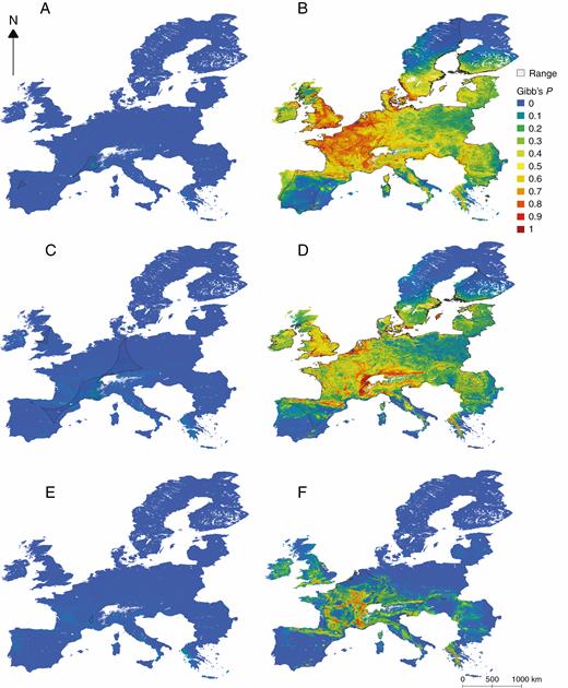
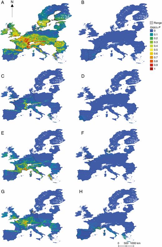
Habitat suitability maps of two allogamous Epipactis species, (A) E. fageticola and (B) E. helleborine, two facultative autogamous species, (C) E. dunensis and (D) E. palustris, and two autogamous species, (E) E. albensis and (F) E. muelleri in Europe, predicted by Maxent using occurrence and environmental data, overlain with α-hulls demonstrating the species’ current realized occurrence. High Gibb’s P-values (in red and orange) represent more suitable habitat conditions where the probability of species presence is higher, while low values (in blue and green) represent lower habitat suitability and occurrence probability. See Appendix 1 for the habitat suitability maps of the remaining species.
Environmental variables contributed to mean Epipactis habitat suitability to different degrees (χ2 = 54.31, d.f. = 8, P < 0.001). The mean contributions of bedrock (26.78 ± 1.41) and land cover (32.07 ± 5.39) were both higher than those of elevation (3.53 ± 1.27), precipitation (6.95 ± 1.81), soil biochemical components (4.00 ± 1.04 and 5.02 ± 2.25) and the second soil physical component (1.72 ± 0.58), and bedrock was also higher than temperature (11.33 ± 3.37) and the first soil physical component (8.61 ± 2.01). Broad-leafed forest, coniferous forest and non-irrigated arable land were dominant land types associated with species occurrence. Of the bedrock types, limestone was associated with most species, and boulder clay was also commonly utilized.
The unweighted average linkage agglomerative clustering method was used to group species based on habitat similarity. Three species clusters were created based on similarities in habitat variables (Fig. 2). Cluster 1 was most distinguishable in terms of variable contributions, having a significantly stronger association with land cover and a weaker association with temperature than the other two groups (Table 2). Cluster 2 had a stronger association with the second biochemical soil component (pH and potassium concentration) than cluster 1, although this difference was of only marginal significance. The mean range size of species in cluster 1 (19.44 ± 6.35 dd) was significantly smaller than that of cluster 2 (P = 0.011; 870.76 ± 48.17 dd). Cluster 1 had a mean habitat suitability probability (0.004 ± 0.001) that was lower than that of cluster 2 (P < 0.001; 0.292 ± 0.03) and cluster 3 (P < 0.001; 0.058 ± 0.025). Cluster 2 had a higher Levins’ B value (niche breadth) (0.58 ± 0.042) than cluster 1 (P = 0.016; 0.185 ± 0.015) and cluster 3 (P = 0.008; 0.182 ± 0.049). There were no differences in mean B2 niche breadth among clusters (P = 0.705).
Differences in mean environmental variable contribution among three species clusters (C1, C2 and C3)
| Environmental variable | P-value | F statistic | Post-hoc pairwise tests P-values | Mean % contribution (s.e.) | |||||||
|---|---|---|---|---|---|---|---|---|---|---|---|
| C1–C2 | C1–C3 | C2–C3 | C1 | C2 | C3 | ||||||
| Bedrock | 0.067 | 3.483 | 0.225 | 0.553 | 0.057 | 26.308 | (2.283) | 19.404 | (3.220) | 29.223 | (1.177) |
| Land cover | 0.002 | 11.120 | 0.002 | 0.317 | 0.008 | 55.439 | (3.546) | 4.186 | (2.903) | 23.345 | (3.307) |
| Elevation | 0.348 | 1.163 | 5.474 | (3.147) | 5.338 | (0.913) | 1.619 | (0.581) | |||
| Precipitation | 0.165 | 2.134 | 1.958 | (1.102) | 11.547 | (4.216) | 9.209 | (2.617) | |||
| SBPC1 | 0.636 | 0.472 | 3.219 | (1.436) | 6.478 | (2.726) | 3.842 | (1.536) | |||
| SBPC2 | 0.057 | 3.759 | 0.048 | 0.661 | 0.114 | 0.538 | (0.283) | 22.269 | (1.486) | 3.291 | (2.314) |
| SPPC1 | 0.029 | 4.977 | 0.727 | 0.073 | 0.058 | 4.707 | (1.385) | 0.730 | (0.064) | 13.642 | (2.745) |
| SPPC2 | 0.857 | 0.157 | 1.238 | (0.509) | 0.863 | (0.187) | 2.312 | (1.053) | |||
| Temperature | 0.002 | 12.430 | 0.004 | 0.004 | 0.483 | 1.119 | (0.493) | 29.187 | (5.329) | 13.516 | (4.313) |
Mean contribution values in bold are significantly higher than those in italics of the same environmental variable.
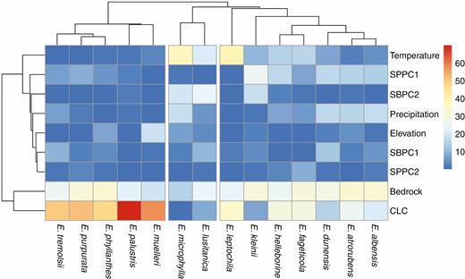
Epipactis species clustered based on habitat similarity. Red and orange cells represent strong associations between species occurrence and the corresponding environmental variable, while blue cells represent weak associations. Variables tested were mean annual temperature, two axes of a PCA of soil biochemical variables (SBPC1 and 2), two axes of a PCA of physical soil characteristics (SPPC1 and 2), elevation, annual precipitation, dominant bedrock material and land cover (CLC).
Among mating systems, there was no significant difference in mean geographical range (F = 1.34, d.f. = 2, P = 0.30), habitat suitability (F = 0.35, d.f. = 2, P = 0.71), Levins’ B niche breadth (F = 0.04, d.f. = 2, P = 0.96) or B2 niche breadth (F = 3.19, d.f. = 2, P = 0.081), but autogamous species demonstrated notably low variation in these measures compared with the other mating systems (Fig. 3).
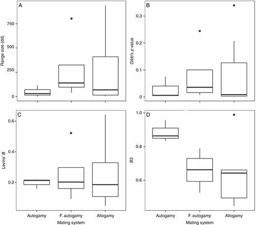
Differences in probability of occurrence, distribution range and niche breadth among autogamous, facultative autogamous and allogamous Epipactis species. F. autoamy, facultative autogamy.
The degree of niche overlap (Schoener’s D) varied between 0.348 (E. purpurata–E. phyllanthes) and 0.817 (E. helleborine–E. palustris) (mean D = 0.550 ± 0.0946) (Table 3; Fig. 4). No difference in mean niche overlap value was detected when comparing among species pairs (i.e. allogamous–allogamous overlap, allogamous–autogamous overlap, etc.; F =0.53, d.f. = 5, P = 0.75). Epipactis helleborine, E. palustris, E. muelleri, E. dunensis, E. leptochila, E. fageticola and E. lusitanica had niches that were closer to the mean ecological niche, while E. microphylla, E. purpurata, E. kleinii, E. tremolsii, E. albensis and E. phyllanthes had more distinctive niches (Fig. 4).
Schoener’s D values representing niche overlap between Epipactis species for all species pairs
| Species | E. atrorubens | E. dunensis | E. fageticola | E. helleborine | E. kleinii | E. leptochila | E. lusitanica | E. microphylla | E. muelleri | E. palustris | E. phyllanthes | E. purpurata | E. tremolsii |
|---|---|---|---|---|---|---|---|---|---|---|---|---|---|
| E. albensis | 0.586 | 0.443 | 0.505 | 0.495 | 0.446 | 0.517 | 0.527 | 0.380 | 0.489 | 0.480 | 0.529 | 0.460 | 0.591 |
| E. atrorubens | 1.000 | 0.589 | 0.621 | 0.639 | 0.772 | 0.538 | 0.621 | 0.706 | 0.505 | 0.691 | 0.777 | 0.539 | 0.558 |
| E. dunensis | x | 1.000 | 0.708 | 0.711 | 0.526 | 0.588 | 0.607 | 0.457 | 0.663 | 0.654 | 0.537 | 0.465 | 0.491 |
| E. fageticola | x | x | 1.000 | 0.683 | 0.611 | 0.532 | 0.665 | 0.476 | 0.639 | 0.663 | 0.500 | 0.464 | 0.556 |
| E. helleborine | x | x | x | 1.000 | 0.513 | 0.593 | 0.704 | 0.468 | 0.694 | 0.817 | 0.521 | 0.539 | 0.476 |
| E. kleinii | x | x | x | x | 1.000 | 0.424 | 0.519 | 0.450 | 0.476 | 0.494 | 0.437 | 0.449 | 0.580 |
| E. leptochila | x | x | x | x | x | 1.000 | 0.525 | 0.486 | 0.646 | 0.598 | 0.520 | 0.463 | 0.509 |
| E. lusitanica | x | x | x | x | x | x | 1.000 | 0.482 | 0.627 | 0.695 | 0.580 | 0.523 | 0.548 |
| E. microphylla | x | x | x | x | x | x | x | 1.000 | 0.515 | 0.470 | 0.382 | 0.447 | 0.481 |
| E. muelleri | x | x | x | x | x | x | x | x | 1.000 | 0.723 | 0.565 | 0.538 | 0.518 |
| E. palustris | x | x | x | x | x | x | x | x | x | 1.000 | 0.517 | 0.506 | 0.467 |
| E. phyllanthes | x | x | x | x | x | x | x | x | x | x | 1.000 | 0.348 | 0.578 |
| E. purpurata | x | x | x | x | x | x | x | x | x | x | x | 1.000 | 0.485 |
Values closer to 1 indicate a high level of overlap, while low values indicate a low level of overlap.
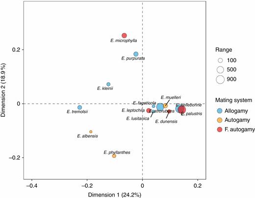
Correspondence plot of Epipactis species niche overlap showing niche similarity among mating systems and in relation to geographic range size. Species with points closer together have higher niche overlap. F. autoamy, facultative autogamy.
DISCUSSION
With the use of ecological niche models (ENMs) and α-hull range definition, we characterized the ecological niches of 14 Epipactis species to test the hypothesis that range size and niche breadth were related to mating system. Epipactis is a terrestrial orchid genus that contains a wide range of allogamous, facultative autogamous and full autogamous species (Claessens and Kleynen, 2011). Epipactis species occupy a wide variety of soils and habitat types, and differ substantially in distribution area in Europe, with some species having very broad ranges (e.g. E. helleborine, E. atrorubens and E. palustris) and others having very narrow distribution ranges (e.g. E. albensis and E. lusitanica), making it a perfect genus to test the impact of mating system on distribution range and niche breadth. Our results showed that mating system did not affect range size, habitat suitability or niche breadth of Epipactis species, supporting earlier findings that mating system does not always predict niche breadth (Johnson et al., 2014; Park et al., 2018, but see Randle et al., 2009; Grant and Kalisz, 2020). However, variation in niche parameters was much wider in facultative autogamous and allogamous species than in autogamous species, which showed very little variation.
The effect of mating system on niche parameters
Selfing species generally have a lower genetic diversity than outcrossing species (Hamrick and Godt, 1996; Honnay and Jacquemyn, 2007) which, in turn, may restrict the ability of selfing species to adapt to local environmental conditions and therefore lead to small ranges and narrow niche breadths. Epipactis is not different in this respect. Population genetic studies have shown that autogamous species tend to have low levels of population genetic diversity (Ehlers and Pedersen, 2000; Squirrell et al., 2002; Hollingsworth et al., 2006; Sramkó et al., 2019). For example, populations of E. dunensis, E. leptochila and E. muelleri have been shown to be completely homozygous and uniform for all loci studied (Squirrell et al., 2002). Similarly, Ehlers and Pedersen (2000) showed that the obligate autogamous E. phyllanthes was completely monomorphic at all loci examined, while the allogamous and widespread E. helleborine showed high levels of polymorphism. However, despite these large differences in genetic diversity between autogamous and allogamous Epipactis species, our results did not show significant differences in niche breadth between mating systems. Nonetheless, huge variation in distribution range and niche breadth was observed among facultative autogamous and allogomous species, while this was less the case for autogamous species. Considering that Epipactis autogams transition from allogams (Brys and Jacquemyn, 2016; Sramkó et al., 2019), it is possible that the larger ranges that are sometimes associated with facultative autogamous species reflect a temporary stage in the transition from outcrossing to selfing and that selfing species will ultimately have more restricted niches than allogamous species (Park et al., 2018), but this would require further investigation to ascertain. Additionally, although the differences in B2 niche breadth among mating mating systems were not significant, our results indicate that autogamous species may prove to have wider niche breadths in environmental space than facultative autogamous or allogamous species.
Selfing can also act as a reproductive barrier (Brys et al., 2014, 2016), and therefore reduce the influx of maladaptive genes and increase the rate of adaptive evolution (Levin, 2010). If orchid seeds arrive in a novel habitat and manage to establish, selfing can be expected to maintain these pre-adapted genotypes and consequently conserve a wider niche breadth of the species. However, this assumes that seeds from a single species are able to colonize multiple habitats. This is not necessarily the case, because seed germination in orchids strongly depends on mycorrhizal fungi, and these fungi may represent an important bottleneck in the colonization process (Bidartondo and Read, 2008; Swarts et al., 2010; Dearnaley et al.,2012, but see Těšitelová et al., 2012). On the other hand, local adaptation can be expedited by low or moderate levels of gene flow by increasing additive genetic variance and allowing post-colonization local adaptation (Peterson and Kay, 2015). Facultative allogamous species may therefore be more likely to experience niche shifts than fully autogamous species. Our results are somewhat in line with this hypothesis, as facultative autogamous species displayed larger variation in range size and niche breadth than autogamous species.
Environmental variables affecting the distributions of Epipactis
To model the niche of each orchid species, we included a wide range of different variables that previously have been shown to influence the distribution of orchids (Bowles et al., 2005; Tsiftsis et al., 2008; McCormick et al., 2009; Acharya et al., 2011; Djordjević et al., 2016; Štípková et al., 2017). These variables related to temperature and precipitation, soil, land cover type, bedrock and elevation. Land cover and bedrock appeared to be the most important variables for predicting mean species habitat suitability. These results are largely in line with previous studies that have modelled the distribution of Epipactis species. For example, Tsiftsis et al. (2008) concluded that in Macedonia, the most important environmental variables linked to orchid occurrence were habitat types. Similarly, Djordjević et al. (2016) showed that temperature and bedrock were important predictors of mean Epipactis occurrence, and certain species such as E. helleborine and E. lusitanica demonstrated strong associations with mean annual temperature. However, the contributions of these variables to differences in habitat suitability and niche breadth were not related to mating system. These results are in contrast to findings of Grant and Kalisz (2020), who showed that the environmental variables that contributed most to differences in niche breadth between selfing and outcrossing species were precipitation, seasonality and elevation. Their results showed that average annual precipitation was higher in outcrossing species, suggesting that selfing species are generally more tolerant to dry or water-limited environments, while selfing species occurred at higher elevations than outcrossing species. None of these variables, however, appeared to have a large influence on the distribution of Epipactis species.
The Epipactis species with wider niche breadths in geographic space tended to have larger geographic ranges than those with narrow niche breadths. This pattern was clear even with though data limitations resulted in measures of geographic range being conservative, especially for the species with large ranges. The greater number of habitats that generalists are able to use allows them to disperse farther than species specialized to inhabit a small number of environments, a pattern that can be seen in the distributions of many taxa (Thompson et al., 1999; Slatyer et al., 2013; Yu et al., 2017). However, in terms of environmental space, the Epipactis species with wide niches did not necessarily have large ranges. Species with large ranges can have narrow niches if they are adapted to habitats that happen to be common in the study area, and species with small ranges can have narrow niches if they are limited by factors other than those included in their niche definition (e.g. geographical barriers) (Peterson et al., 2011; Saupe et al., 2015). Most of the Epipactis species with small ranges demonstrated distinctly strong associations with forests, and the dependence on forests that they developed in their evolutionary histories may have made them less able to utilize other environments, limiting their ranges. The existence of both forest-dependent and generalist Epipactis species indicates that there may be some species traits not investigated in this study which affect their distributions.
Other factors contributing to Epipactis distributions
An aspect of Epipactis niches that should be investigated to create a clearer picture of the drivers of their distributions is the influence of biotic interactions, in particular with mycorrhizal fungi. The lack of an endosperm in orchid seeds means that terrestrial orchids need fungi in the soil to germinate and establish (Smith and Read, 2010), and therefore the presence of fungal species that provide nutrients for developing seeds probably restricts Epipactis distributions (Ogura-Tsujita and Yukawa, 2008; McCormick and Jacquemyn, 2014). Species that are capable of associating with a wide variety of mycorrhizal fungi can be expected to have a wider distribution range and niche breadth than species that associate with a small number of fungi. For example, the widespread E. helleborine and Gymnadenia conopsea have recently been shown to associate with a wide range of orchid mycorrhizal fungi across their entire distributions, and their mycorrhizal partners differed substantially between geographic regions (Xing et al., 2020). Associating with different sets of mycorrhizal fungi can also induce niche differentiation (Jacquemyn et al., 2014, 2015) and act as a reproductive barrier in a similar way to selfing. For example, Jacquemyn et al. (2016) showed that Epipactis species of dune and forest habitats associated with distinct mycorrhizal communities and that these differences in mycorrhizal communities severely limited gene flow between the two habitats (Jacquemyn et al., 2018). Immigrant seeds had a significantly lower probability of protocorm formation than native seeds. Hybrid seeds originating from crosses between the two ecotypes also showed significantly lower protocorm formation than pure seeds, further contributing to reproductive isolation. These results suggest that differences in niche breadth may also be caused by differences in mycorrhizal associations. Furthermore, the cluster of species characterized by having small ranges in our results had strong associations with forest land cover, and Bidartondo and Read (2008) concluded that mycorrhizal fungi that are restricted to forests limit the dispersal of their orchid symbionts. However, Těšitelová et al. (2012) found that neither the availability of mycorrhizal fungi nor abiotic habitat conditions limited germination in Epipactis, even in species that demonstrate habitat specializations in adulthood. Further research therefore is needed regarding both seedlings and adult plants to see whether species with narrow niche breadths in mycorrhizal associations have significantly smaller distribution ranges than species with broad niche breadth in mycorrhizal partners.
Conclusion
To conclude, our results do not support the hypothesis that autogamous species have larger ranges and wider ecological niches than facultative autogamous or allogamous species. For Epipactis species in Europe, bedrock and land cover type appeared to be more important environmental variables than climatic conditions in predicting distributions. This suggests that plant traits other than mating system are more important in defining the ecological niche of Epipactis species. Because germination and seedling establishment are critical stages in the life cycle of orchids, differences in interaction with mycorrhizal fungi may be as, or more, important than mating system in defining the distribution range and niche breadth of orchids. Future research should investigate in more detail that, in addition to abiotic environmental structure, biotic interactions such as those with mycorrhizal fungi are important drivers of Epipactis distributions.
SUPPLEMENTARY DATA
Supplementary data are available online at https://dbpia.nl.go.kr/aob and consist of File S1: the cleaned species location data before aggregation .
FUNDING
This work was supported by the Flemish Fund for Scientific Research [G093019N].
LITERATURE CITED
Habitat suitability maps overlain with α-hull range estimations of Epipactis species not illustrated in Fig. 1: E. muelleri (A), kleinii (B), leptochila (C), lusitanica (D), microphylla (E), tremolsii (F).
