


Abstract
Large, persistent seed banks contribute to the invasiveness of non-native plants, and maternal plant size is an important contributory factor. We explored the relationships between plant vegetative size (V) and soil seed bank size (S) for the invasive shrub Ulex europaeus in its native range and in non-native populations, and identified which other factors may contribute to seed bank variation between native and invaded regions.
We compared the native region (France) with two regions where Ulex is invasive, one with seed predators introduced for biological control (New Zealand) and another where seed predators are absent (La Réunion). We quantified seed bank size, plant dimensions, seed predation and soil fertility for six stands in each of the three regions.
Seed banks were 9–14 times larger in the two invaded regions compared to native France. We found a positive relationship between current seed bank size and actual plant size, and that any deviation from this relationship was probably due to large differences in seed predation and/or soil fertility. We further identified three possible factors explaining larger seed banks in non-native environments: larger maternal plant size, lower activity of seed predators and higher soil fertility.
In highlighting a positive relationship between maternal plant size and seed bank size, and identifying additional factors that regulate soil seed bank dynamics in non-native ranges, our data offer a number of opportunities for invasive weed control. For non-native Ulex populations specifically, management focusing on ‘S’ (i.e. the reduction of the seed bank by stimulating germination, or the introduction of seed predators as biological control agents) and/or on ‘V’ (i.e. by cutting mature stands to reduce maternal plant biomass) offers the most probable combination of effective control options.
INTRODUCTION
The performance of plants in terms of reproduction, growth and persistence in a given ecosystem may differ between their native and non-native ranges. Although many species may not perform better outside their native range (Williamson and Fitter, 1996), some species show higher growth, dispersal or survival rates in the new environment (Mack et al., 2000; Richardson and Pyšek, 2006; Blumenthal and Hufbauer, 2007; Hahn et al., 2012; Lamarque et al., 2014). Others show higher nutrient absorption efficiencies and/or N-fixing symbiosis (Ehrenfeldt, 2003; Funk and Vitousek, 2007; van Kleunen et al., 2010) or increased seedling heights and biomass (Henery et al., 2010). Differences in reproductive traits have also been reported, and can include an extended reproduction period (Barrett et al., 2008), higher reproductive outputs (Rejmánek, 1996; Grigulis et al., 2001; Henery et al., 2010; Correia et al., 2015) or a different seed mass (Hierro et al., 2013).
Among reproductive traits promoting invasiveness, the similarity of floral traits to existing native species in introduced areas (Gibson et al., 2012) and the formation of large and persistent seed banks have been reported (Witkowski and Wilson, 2001; Krinke et al., 2005; Witkowski and Garner, 2008). Large seed banks can be both a symptom and a cause of invasiveness, but will influence the persistence of an established species within a location (Baskin and Baskin, 2001; Gioria et al., 2012). The failure of some control programmes can be explained by the failure to take into account the state and dynamics of the soil seed bank (Milakovic and Karrer, 2016; Williams et al., 2016). More specifically, the capacity to form large seed banks should be taken into account when considering invasive leguminous trees and shrubs, as has been outlined for Australia and South Africa (Paynter et al., 2003; Richardson and Kluge, 2008; Gibson et al., 2011).
Although several authors have suggested that reproductive traits could promote invasiveness through increasing seed bank size (Krinke et al., 2005; Witkowski and Garner, 2008; Gioria et al., 2012), very few studies have compared seed bank size for a species between its native and non-native ranges using a single observation framework. The study of Fowler et al. (1996) on the leguminous shrub Cytisus scoparius revealed no differences in seed bank size between the native and the invaded zones. In contrast, Herrera et al. (2011) reported that the density of seeds in the soil for the leguminous shrub Genista monspessulana was 15 times larger in its invaded area (California, USA) compared to its native region (Mediterranean Basin, France). Compiling seed bank data from different studies for a range of Acacia species native to Australia (Weiss, 1984; Auld, 1986) and invasive in South Africa (Holmes et al., 1987; Strydom et al., 2017) showed smaller seed banks in the native range (4–3600 seeds m−2) than in the invaded range (1017–45 800 seeds m−2). Whether the invasive character of a given species is related to differences in seed bank size or not, and which factors influence such a relationship, remains underexplored.
These factors may be related to: (1) higher seed production in the non-native range, or to higher allocation of resources to reproduction by mature individuals (Rejmánek, 1996; Herrera et al., 2011), (2) pre-dispersal seed predation with release from seed predators in the non-native range (Keane, 2002) and (3) seed accumulation in soil (linked to differences in post-dispersal seed predation, dormancy of seeds, germination rate, secondary dispersal, and the biotic or abiotic environment in soils; Grigulis et al., 2001; Hill et al., 2001). For example, in Genista monspessulana, Herrera et al. (2011) highlighted that the larger soil seed bank in the invaded region is correlated with plants being taller, denser and older, suggesting differences in seed production by these plants. This could also be the result of the evolution of more competitive individuals with a higher growth rate and longevity, after release from enemy pressure (Blossey and Notzold, 1995; Hierro et al., 2005).
In this study, we focused on common gorse, Ulex europaeus, a leguminous shrub considered as a major invasive pest outside its native range (Lowe et al., 2000). Common gorse is becoming a model species in invasion science (Kueffer et al., 2013) and its known biological characteristics will contribute to our analysis. It has frequently been declared a successful invasive species due to its growth and reproductive performance. Common gorse produces large numbers of seeds and has soil seed banks, which persist for up to 20 years (Hill et al., 2001; Gonzalez et al., 2010). It develops in patches with high stem densities, fast growth and high biomass production; it can resprout from stumps, features a high nutrient capture and has the ability to fix nitrogen through symbiosis (Lee et al., 1986; Clements et al., 2001; Hill et al., 2001). Moreover, in some regions where it was introduced, gorse has adapted to local conditions, through higher seedling growth rates (Hornoy et al., 2011), a higher seed mass (Atlan et al., 2015a; Udo et al., 2017), a faster germination rate and a reduction of integumentary dormancy (Udo et al., 2017). The size of the soil seed bank was reported to be systematically smaller in its native range (Puentes et al., 1988; Gonzalez et al., 2010) than in invaded regions, as demonstrated in previous studies (Moss, 1959; Ivens, 1978; Zabkiewicz and Gaskin, 1978; Rees and Hill, 2001).
To identify the factors responsible for possible differences in soil seed banks between native and invaded regions, we used and extended the framework proposed regarding the relationship between plant size and reproductive output [i.e. reproductive output (R) – vegetative tissues (V) relationships, see Klinkhamer et al., 1992; Sugiyama and Bazzaz, 1998; Weiner et al., 2009a]. We propose an extension to this framework to include relationships between seed bank size (S) and vegetative tissues (V) (hereafter referred to as the ‘SV relationships’). To this end, we collected plant and seed bank data from three geographical regions: the native region (France) and two regions where the species is invasive, one with introduced seed predators for biological control (New Zealand) and one where seed predators were absent (La Réunion). Theoretical expected SV relationships are presented in Fig. 1. Three of them (Fig. 1A–C) show a positive relationship between basal area and seed bank size, while the last one (Fig. 1D) shows no relationship. Positive relationships exist between plant size and reproductive output (Weiner et al., 2009a) and this was confirmed for gorse (Delerue et al., 2013). When a positive SV relationship exists, it implies that recent and present plant size and therefore recent and present seed production contribute significantly to the seed bank composition. Otherwise, it implies that the relationship is broken after seed production (i.e. during the stages of pre-dispersal predation or seed accumulation in the soil) or that the seed bank is more dependent on seed production of the gorse population in the long term and is little influenced by present seed production and present gorse population characteristics (Fig. 1D). With respect to positive SV relationships, in their most simple representation, seed bank size increases because plants are larger in non-native contexts, and produce more seeds (Fig. 1A). In the second and third cases (Fig. 1B, C), for gorse plants of the same size, a higher proportion of resources captured by the plants (carbohydrates and nutrients) is invested in the production of seeds (Weiner et al., 2009a), which are successfully incorporated into the seed bank. It modifies SV relationships with a change of intercept (Fig. 1B) or slope (Fig. 1C) as in Sugiyama and Bazzaz (1998, fig. 1). These three cases (Fig. 1A–C) are not exclusive. Plants could be larger in a non-native context as in Fig. 1A, and modifications of the intercept (Fig. 1B) and slopes (Fig. 1C) could also occur (see Weiner et al., 2009b, fig. 4 for an illustration regarding RV relationships with modifications of both plant size and intercept). Regarding the patterns described in Fig. 1B and C, two main mechanisms leading to such patterns can be proposed. First, release from seed predators compared to native environments (Keane, 2002) could be involved. This is especially relevant for La Réunion where seed predators are absent. In the case of introduction of seed predators for biological control, the proportion of seeds destroyed by the predators (Hill et al., 1991; Davies et al., 2008) is lower compared to in France (Delerue et al., 2014). Secondly, changes in the allocations to reproduction in resource-rich environments have also been reported in the literature with higher allocation at higher soil fertility (e.g. Weiner et al., 2009b). Gorse in native areas is characteristic of acidic nutrient-depleted heathlands (Demounen, 1979; Augusto et al., 2010; Delerue, 2013). In invaded areas, it can be found on a wide diversity of substrata including volcanic soils and in agricultural land (Lee et al., 1986, Hill et al., 2001 for New Zealand; Richardson and Hill, 1998 for Australia), suggesting potential differences in soil fertility for some non-native populations. This could create potential for higher allocation to reproduction, contributing to higher seed bank provisioning. Our overarching hypothesis was that positive SV relationships exist (higher seed bank densities for plants of greater dimensions) and can be used to explain the patterns in seed banks and plant size in native and invaded regions. More specifically, we assumed that three possible patterns could explain the higher seed bank densities in non-native contexts. First, differences in plant development between native and invaded regions will lead to differences in seed bank size (Fig. 1A). Secondly, for plants of the same size, seed banks could be better supplied (Fig. 1B or C). This could be due to the absence (La Réunion) or lower activity (New Zealand) of seed predators or to higher seed production in the case of higher soil fertility in the invasive context. Thirdly, a combination of these different patterns is also possible.
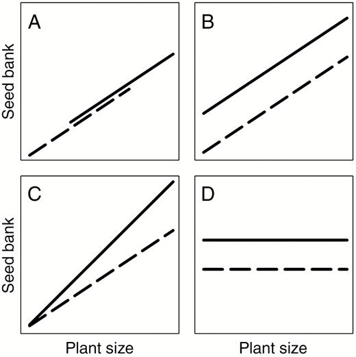
Possible SV relationships between plant size and seed bank size. A higher seed bank size is considered in non-native (solid lines) compared to native (dotted lines) areas. Note that linear relationships are presented. In agreement with earlier work regarding plant size and reproductive output, the SV relationships are not necessarily linear but data can be transformed to linearize the relationships. (A) The case of ‘bigger’ plants in non-native areas as an explanation of higher seed banks. (B,C) Plants of the same size produce higher amounts of seeds incorporated into the seed bank. The reasons for this pattern can be three-fold: (1) a higher proportion of resources is devoted to seed production; (2) a lower proportion of the seeds is destroyed by seed predators prior to primary dispersal; and (3) a lower proportion of the seeds disappears from the seed bank in the soil. These modifications of the baseline SV relationship presented in A can result in a difference of intercept (B, modifications are constant for the entire range of plant dimensions) or slope (C, the nature of the relationship has changed and modifications are larger for larger individuals) (see Sujiyama et al., 1998, figure 1 for similar changes in RV relationships). Simultaneous effects due to a change of plant size as in A, and a change of intercept (B) or slope (C) are possible (see Weiner et al., 2009b, figure 4 for an illustration regarding RV relationships) but not represented here. (D) The absence of an SV relationship. This can result, for example, from the accumulation and persistence of seeds in the seed bank over a long time, while stand characteristics and basal area change.
MATERIALS AND METHODS
Study species
Common gorse, Ulex europeaus L. (Genisteae, Fabaceae), is native to the European Atlantic coast. It is a spiny shrub, with reports stating maximum heights of 4–7 m and maximum ages of 15–30 years (Moss, 1959; Lee et al., 1986; Hill et al., 1996; Rees and Hill, 2001). In New Zealand, seed production ranged from 442 to 36 741 seeds m−2 year−1 but due to predation by seed weevils, the actual seed rain was lowered to 265–2939 seeds m−2 year−1 (Rees and Hill, 2001). Seed bank densities in topsoils for invaded regions ranged from 200 to 37 000 seeds m−2 (Moss, 1959; Ivens, 1978; Zabkiewicz and Gaskin, 1978; Rees and Hill, 2001) and this was higher than the reported values of 503–1312 seeds m−2 for native contexts in Spain, the UK and France (Puentes et al., 1988; Mitchell et al., 1998; Gonzalez et al., 2010). Due to the autochorous character of the species, when studying seed dispersion around an isolated gorse shrub, Hill et al. (1996) found that 50 % of the seeds fall within 1 m of the parent plant, and 80 % within 2 m. In dense tickets, branches are intertwined and dispersion distance may be even lower. Seed banks are reported to be long lasting and some may persist for decades; at shallow depths, however, the majority of the seeds remain in the soil for less than 10 years (Hill et al., 2001). Germination of seeds and seed death are the most important processes leading to the depletion of the soil seed bank but the relative importance of both processes is difficult to assess (Rees and Hill, 2001).
The species was introduced intentionally in New Zealand (before 1835) and in La Réunion (in 1825) (Atlan et al., 2015b). Flowering typically occurs once a year – in spring – in its native region (with some individuals flowering year-round). In invaded regions, several flowering periods may exist. In La Réunion, flowering lasts 10 months with a peak in winter. In New Zealand, seed production is bivoltine and can occur both in autumn and in spring (Hill et al., 1996, 2001), even though spring flowering produces many more seeds (Hill et al., 1991; Atlan et al., 2010). In New Zealand, specific pre-dispersal seed predators, the gorse seed weevil (Exapion ulicis) and the gorse pod moth (Cydia succedana), were introduced as biocontrol agents, in 1931 and 1992, respectively. These biological control agents are absent from La Réunion Island (Hill et al., 2008). The larvae of these two seed predators infest pods prior to seed rain. Both lay eggs in spring, so that seed predation is only effective in this season (Hill et al., 1991). Seed predation can eliminate 30–80 % of the total annual seed production in France (Atlan et al., 2010; Delerue et al., 2014). It is highly variable in New Zealand (from 10 to 90 %) depending on the gorse and seed predators’ phenology (Hill et al., 1991, 2000; Gourlay et al., 2003; Sixtus et al., 2006).
Site description
Six sites were established in each of the following geographical regions: France, New Zealand and La Réunion. Altitudes above sea level varied from close to sea level in France and New Zealand, to nearly 2000 m in La Réunion (Table 1). Fieldwork was carried out in 2013 at the end of the main reproductive season, i.e. in June–July for France, January–February for New Zealand and October–December for La Réunion. The sites sampled were chosen to reflect the range where the species occurs naturally in the three regions (Table 1). First, they were geographically stratified within each region, and then randomly selected from the potential sites in each geographical sub-region; site characteristics were also considered (see below). In France, this gave two sites in each of three separate sub-regions close to the Atlantic coast, for New Zealand two on North Island, two on South Island close to the coast and two more on inland hilly slopes, and for La Réunion a more regular distribution across all the populations present on the island. Site selection was made to ensure, as far as possible, general homogeneity regarding the main stand characteristics. All sites were situated on fairly flat terrain (slopes <5 %) and in full sunlight (no stands were under forest canopy). We focused on the homogeneity of the gorse thickets relative to the canopy (closed canopy), stem density (regularly distributed) and height of the individuals (limited differences between stems). Closed canopies were selected because most seeds were shown to fall within this canopy, and even 59 % within 1 m of the pod (Hill et al., 1996), permitting a priori a closer relationship between gorse plants and localized seed banks. In the case of irregular canopies, which occur in all three regions, in particular along the advancing front of the gorse thickets, or when the stands become older and senescent, seed rain could disperse the seeds further away from each individual. This could make it more complicated to relate plant dimensions to seed bank size. We have no a priori expectation relative to the size of the seed bank for gorse thickets with an irregular canopy. As far as landowner knowledge was traceable historically, the dominant land use and the landscape context had not changed in recent decades. The age of the gorse stands ranged between 5 and 15 years (Table 1) based on owner information, growth ring counts and average annual diameter growth (Lee et al., 1986; Augusto et al., 2005).
Description of the sites sampled in France, New Zealand and La Réunion.
| Site ID | Site name | Latitude | Longitude | Altitude (m) | MATa (°C) | MAPa (mm) | Sampling | Stand age (years)j |
|---|---|---|---|---|---|---|---|---|
| France | ||||||||
| FR1b | St Michel de Rieufret | 44.37°N | 0.27°W | 60 | 12.4 | 930 | 11/06/2013 | 7–9 |
| FR2c | Salles - La Caplanne | 44.33°N | 0.56°W | 23 | 12.5 | 1020 | 14/06/2013 | 7–8 |
| FR3d | St Pée sur Nivelle | 43.23°N | 1.32°W | 100 | 12.5 | 1195 | 17/06/2013 | 13–15 |
| FR4e | Ascain | 43.20°N | 1.35°W | 219 | 11.9 | 1269 | 18/06/2013 | 8–10 |
| FR5f | Monterfil | 48.03°N | 2.00°W | 90 | 10.9 | 762 | 01/07/2013 | 5–9 |
| FR6f | Paimpont | 47.60°N | 2.13°W | 157 | 11.5 | 785 | 02/07/2013 | 9–11 |
| New Zealand | ||||||||
| NZ1g | Matata | 37.53°S | 176.43°E | 260 | 13.9 | 1574 | 09/01/2013 | 5–8 |
| NZ2g | Mamaku | 38.02°S | 176.03°E | 560 | 11.5 | 2066 | 10/01/2013 | 12–14 |
| NZ3g | Pines beach_poplar | 43.21°S | 172.41°E | 5 | 11.2 | 804 | 11/02/2013 | 14–15 |
| NZ4g | Pines beach_inside | 43.22°S | 172.41°E | 5 | 11.2 | 804 | 14/02/2013 | 8–10 |
| NZ5g | Torless farm_S | 43.17°S | 171.54°E | 519 | 6.9 | 1906 | 27/02/2013 | 8–11 |
| NZ6g | Torless farm_N | 43.17°S | 171.55°E | 550 | 6.9 | 1906 | 28/02/2013 | 8–9 |
| La Réunion | ||||||||
| LR1h | Maido | 21.06°S | 55.37°E | 1836 | 15.3 | 1745 | 05/11/2013 | 5–6 |
| LR2i | Champs de Foire (PDC) | 21.20°S | 55.59°E | 1640 | 16.7 | 1636 | 21/10/2013 | 9–10 |
| LR3e | Sicalait (PDC) | 21.22°S | 55.58°E | 1618 | 16.7 | 1636 | 22/10/2013 | 5–6 |
| LR4g | Piton de l’eau | 21.18°S | 55.69°E | 1988 | 17 | 1620 | 10/12/2013 | 8–9 |
| LR5e | Montvert | 21.28°S | 55.60°E | 1579 | 16.7 | 1636 | 28/11/2013 | 5–6 |
| LR6g | Calistemon | 21.28°S | 55.58°E | 1330 | 16.7 | 1636 | 21/11/2013 | 6 |
a World Clim database: http://worldclim.org/bioclim; MAT, mean annual temperature; MAP, mean annual precipitation.
b Present land use ‘edge of forest’; c ‘open forest’; d ‘edge with meadow’, e ‘edge of pasture, f ‘edge/heathland’; g ‘pasture’; h ‘road border’, i ‘fallow’, j based on owner information, completed/checked by annual growth ring counts, visual observation of disturbance and average diameter growth (Lee et al., 1986; Augusto et al., 2005).
Gorse harvest and stem inventory
At each site, we established three adjacent strips of six gorse plots of 1 m2 each (3 × 6 = 18 m2 in total). All mature and reproducing shrubs (i.e. >40 cm tall; Delerue, 2013) were considered within the plots. We counted the number of stems, and for each stem, its total length and diameter at 10 cm from the soil surface were measured. We also measured the height of the tallest stem. Then a set of descriptors was computed at the plot–m2 level (basal area, stem density, average plant height) and at the site level (by averaging the data of the 15 interior 1-m2 plots). To avoid edge effects, the three border plots were withdrawn for this calculation. Gorse stems were cut and removed, both to facilitate their measurements and to allow subsequent soil sampling for seed bank assessment. At this stage, growth ring counts were made on the stumps of the largest individuals.
Seed bank assessment
After removal of the gorse shrubs, soil was collected within the four central and internal plots of the 3 × 6 = 18 m2 grid of the gorse thicket. In each of the four plots, the soil was sampled using a soil plug with an internal diameter of 2.1 cm and a length of 5 cm (Niollet et al., 2014). Seed banks were collected from the first 5 cm of the soil because (1) under gorse thickets, the majority of seeds can be found in the topsoil layers in native (Puentes et al., 1988) and non-native areas (Ivens, 1978) and (2) new gorse individuals are produced mainly by seeds that remain in the 0–5 cm topsoil layer (Rees and Hill, 2001). Thirty sampling plugs (for a total of ~104 cm2) were distributed regularly over the entire 1-m2 plot, and pooled into one sample in a plastic bag. The samples were stored in the laboratory at low temperatures (1–4 °C) until processing. We used an elutriation method to determine seed bank size as Gross (1990) demonstrated that it was better than germination methods to study the seed bank size for species with big seeds and a shiny seed coat. When processing, the entire sample was sieved sequentially through several mesh sizes. At each step of the separation, the discarded fraction was scrutinized under optimal light conditions to detect and collect individual seeds of U. europaeus. We then calculated the corresponding seed bank density per plot (seeds m−2) from the number of seeds found for 104 cm2 of soil sampled per m2 (30 seed plugs per plot). Finally, we calculated the mean seed bank density for each site based on the values of the four sampled plots.
Viability tests of seeds from the seed bank
Viability tests were performed on subsamples of six seeds per site using a chemical tetrazolium test (Marrero et al., 2007). Two replicates of the test were performed, i.e. a total of 12 seeds were tested for each site. The number of seeds tested was restricted by the smallest available number of seeds from a French site. Seeds were placed between two Whatman filter papers with water in Petri dishes. Once the seeds were sufficiently imbibed, embryos were excised and placed in Petri dishes filled with tetrazolium solution in an oven for 48 h. Coloration of embryos was then noted. A significant proportion of the seeds was still dry after 1 year of the experiment and, for these seeds, the tegument was scarified to boost imbibition of the seeds. The same steps of the test were run after this scarification. The seeds were considered as viable if the embryo was stained red or as non-viable if white or of an ambiguous colour. To interpret the results of the stained seeds, we used known patterns of staining of the embryos (Rao et al., 2006). For more details, see also Gonzalez et al. (2010).
Number of seeds per pod and estimation of pod predation rate
In total, 10–15 distinct mature gorse individuals were selected at each site at the time of seed bank sampling. From these we harvested 30–50 ripe pods from various parts of the upper and outer branches of each gorse shrub. Pods were opened and inspected for seed predation. Either the presence of seed predators (larvae or adult seed weevils or moth larvae) or, in the absence of seed predators, visual observation of destroyed or partially eaten seeds were used to classify the pod as predated as in Delerue et al. (2014). Intact pods were used to assess the number of seeds per pod. Once a pod is infested, the proportion of seeds destroyed in the infested pod is always high and varies little between 80 and 100 %, independently from the type of predator (weevil or moth; Delerue et al., 2014). Thus, we used the number of pods predated over the total number of pods inspected as the metric for seed predation at each site. The number of seeds per pod is known to be fairly constant for a given site (Hill et al., 2001; Atlan et al., 2010), so our estimation for this variable is reliable regarding sampled gorse thickets. However, to determine a precise seed predation rate, the estimation would require several months of monitoring during the entire reproductive season (Delerue et al., 2014). Therefore, the estimations we made regarding pod predation rates have to be considered with caution, but they were important to confirm the absence of seed predators in La Réunion and their presence in the other regions.
Soil properties
Soil samples collected for seed bank assessments were used for soil analysis. One composite sample was prepared per site by mixing aliquots of equal size of the ten plots sampled. Soil pH–H2O was determined in a water/soil suspension with a mass-to-volume ratio of 1 g/2.5 mL. Soil texture was determined by a mechanical dispersion-decantation method providing the following size classes: clay (<0.003 mm), silt (0.003–0.063 mm) and sand (>0.063 mm) (Piper, 1950). Total organic C and N contents were assessed using a dry combustion method with oxygen and a CN analyser. Total P was analysed via a segmented flow analyser after HNO3/HCl digestion. Exchangeable Ca, K, Mg and Na were measured by inductively coupled plasma mass spectrometry after 1 m NH4COOH extraction and the total cation exchange capacity (CEC) was measured by flow injection analysis colorimetry after 1 m NH4COOH extraction (Metson, 1956).
Data analyses and statistics
All analyses were performed with R software (R Core Team, 2016, v.3.2.5).
Regional differences regarding seed bank size, gorse thickets and soil properties
For all six sites per region, we calculated seed bank sizes and gorse thicket characteristics (basal area, stem density and height) by taking the mean of the sampled plots. Soil properties were already available for each site from the composite sample. For all these variables, we used non-parametric Kruskal–Wallis tests to look for potential differences between regions because assumptions of the normality distribution of residuals for parametric ANOVA are difficult to verify with only 18 values (note that parametric ANOVA and non-parametric Kruskal–Wallis procedures gave exactly the same result). Pairwise multiple comparisons were carried out when Kruskal–Wallis tests gave significant results.
SV relationships
Regarding SV relationships, we used the basal area as a relevant proxy for gorse vegetative tissues (Augusto et al., 2009). These relationships were investigated using mean values per site. To compare our empirical data with our theoretical framework (Fig. 1), we performed an ANCOVA to test the global relationship between basal area and seed bank size. Both seed bank densities and basal areas were cube root transformed before analysis to linearize the relationships. Post-hoc analysis to detect differences of intercept and slope between regions was done using pairwise multiple comparisons (multcomp package). Additional analyses concerned the same relationships between basal area, seed bank densities and potential differences of relationships between regions using values measured at the 1-m2 plot level. As the different plots sampled within a site were not independent, the statistical procedure performed involved linear mixed modelling and random permutation tests (see Supplementary Data 1, Fig. S1, for a complete description of this analysis at the plot level).
Soil properties and the Site Fertility Index
We compared soil properties between regions using non-parametric Kruskal–Wallis tests as mentioned above (Supplementary Data 2, Table S1). Moreover, as many soil properties measured were correlated, we performed a principal component analysis to create more synthetic variables that could discriminate sampled soils. The first and second components explained 50 % and 30 % of the variation in soil properties, respectively (Supplementary Data 2, Fig. S2ab). All the main variables contributing to the first component were related to organic matter content and soil fertility. They concerned the total content of major elements for plant nutrition (Ntot and Ptot), total cation exchange capacity (CEC) and organic matter content (Corg). Thus, the first component can be regarded as corresponding to a fertility gradient. The main variables contributing to the second component were related to particle size distribution (proportions of sand, silt and clay) and contents of some cations (mainly Ca and Mg). Thus, this second component was less related to fertility compared to the first one (Supplementary Data 2, Fig. S2b). Based on these results, a Site Fertility Index was derived from the coordinates of the different sites in the first component. Finally, to have a straightforward fertility index, we set the minimal value to zero to have only positive values (see Supplementary Data 2, Fig. S2 for more details regarding soil properties and Site Fertility Index).
To test the possible influence of the Site Fertility Index on seed bank size, while taking into account the expected effect of plant size, a three-step process was implemented. First, we fitted a linear relationship between site mean gorse basal area and site mean seed bank size. Secondly, the model residuals were used to describe the deviation of each site from the general relationship. Finally, we analysed the linear relationship between site deviation and Site Fertility Index.
RESULTS
Seed banks and seed characteristics
The average number of seeds per m2 in soils inside the gorse thickets was significantly higher in non-native regions than in the native region: there were 1375 ± 376 seeds m−2 in France, whereas there were 13 066 ± 3643 seeds m−2 in New Zealand and 19 960 ± 4672 seeds m−2 in La Réunion (Fig. 2A and Table 2). The maximum values for a given plot inside the gorse thicket were 3668 seeds m−2 for France and reached very high values for the invaded areas with 44 275 and 57 636 seeds m−2 in New Zealand and La Réunion, respectively. Seed viability did not differ significantly between regions and ranged from 95.8 to 97.2 % (data not shown; P > 0.05). The percentage of seeds needing scarification after 1 year of experimental testing (step 1, imbibition of the seeds), in order to test viability (step 2, chemical test), was 51.4–70.8 % and this did not differ between regions (P > 0.05). The number of seeds per pod was similar in the three regions with 3.6–4.1 seeds per pod (Table 2), indicating that this reproductive trait cannot influence seed bank densities. Our pod harvest showed no significant differences in pod predation rates between France and New Zealand at the time of the single pod harvest of this study (40 % and 62 % of infested pods, respectively), and confirmed the absence of predation in La Réunion (Table 2).
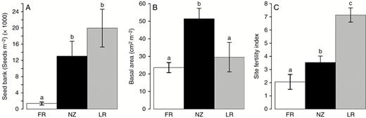
Differences in seed bank (A), basal area (B) and Site Fertility Index (C) between regions. Means ± s.e. of six populations per region. FR: France, NZ: New Zealand, LR: La Réunion. Differences between regions were significant for the three variables (Kruskal–Wallis tests, P < 0.01). Different letters indicate significant differences between regions (post-hoc comparisons).
Differences between regions regarding seed production and seed bank, gorse shrubs and main soil properties related to the soil fertility index.
| France | New Zealand | La Réunion | |||||||||||||
|---|---|---|---|---|---|---|---|---|---|---|---|---|---|---|---|
| Variable | Units | χ2-value (2 ddl) | Mean | ± | s.e. | Mean | ± | s.e. | Mean | ± | s.e. | ||||
| Seed production and seed bank | |||||||||||||||
| Seedbank | seeds m−2 | 11.40 | ** | 1375 | ± | 376 | a | 13 066 | ± | 3643 | b | 19960 | ± | 4672 | b |
| Seeds per pod | seeds per pod | 1.73 | 4.09 | ± | 0.14 | 3.59 | ± | 0.35 | 3.82 | ± | 0.19 | ||||
| Pod predation rate | % | 13.01 | ** | 39.74 | ± | 10.03 | b | 62.39 | ± | 8.06 | b | 0.00 | ± | 0.00 | a |
| Gorse shrubs | |||||||||||||||
| Basal area | cm2 m−2 | 8.57 | ** | 23.61 | ± | 2.87 | a | 51.39 | ± | 5.93 | b | 29.55 | ± | 8.35 | a |
| Density | individuals m−2 | 4.30 | 3.74 | ± | 0.47 | 4.00 | ± | 0.95 | 9.48 | ± | 2.61 | ||||
| Height | cm | 3.70 | ** | 224.4 | ± | 18.6 | 245.1 | ± | 14.9 | 138.9 | ± | 39.5 | |||
| Soil properties | |||||||||||||||
| Corg | % | 11.10 | ** | 5.13 | ± | 0.77 | a | 6.3 | ± | 1.24 | a | 15.93 | ± | 1.71 | b |
| Ntot | % | 10.84 | ** | 0.32 | ± | 0.06 | a | 0.49 | ± | 0.08 | a | 1.15 | ± | 0.15 | b |
| Ptot | ‰ | 12.43 | ** | 0.22 | ± | 0.06 | a | 0.35 | ± | 0.02 | a | 0.97 | ± | 0.15 | b |
| CEC | cmolc kg−1 | 11.59 | ** | 12.58 | ± | 1.78 | a | 20.45 | ± | 4.36 | a | 40.02 | ± | 3.76 | b |
Data measured or calculated for each population were used for analysis (n = 18, 6 populations per region). Results of Kruskal–Wallis tests are shown (χ2-values) as well as their level of significance (**, P < 0.01). Different letters indicate significant differences between regions.
Description of gorse thickets
On average, minimum stem diameters ranged between 5 and 10 mm and maximum stem diameters between 56 and 88 mm, with significantly larger average diameters (means ± s.e.) in New Zealand (9.7 ± 1.6 mm) as compared to France (6.3 ± 1.0 mm) and La Réunion (4.7 ± 2.5 mm). While the density of stems and the height of plants did not differ significantly between regions, gorse thickets showed higher basal areas in New Zealand (51 cm2 m−2) compared to France (23 cm2 m−2) and La Réunion (30 cm2 m−2) (Table 2, Fig. 2B), showing that for our sampled sites, plant biomass able to produce seeds was highest for New Zealand.
Soil properties and Site Fertility Index
All soil properties measured showed significant differences between regions, and values for Corg, Ntot, Ptot and CEC (the main variables contributing to the Site Fertility Index, see Supplementary Data 2, Table S1, Fig. S2) are provided in Table 2. For these four variables, La Réunion had the highest values and France the lowest (Table 2). As a result, the synthetic Site Fertility Index was significantly highest in La Réunion, lowest in France and intermediate in New Zealand (Fig. 3C). Note that other important nutritive elements (K and Mg) were lowest in France, and that pH increased slightly in New Zealand and La Réunion (Supplementary Data 2, Table S1), confirming the higher fertility in La Réunion compared with France.
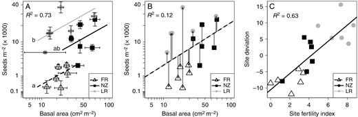
Relationships between seed bank, basal area, region of origin and Site Fertility Index. (A) Model 1: regional SV relationships between seed bank and basal area. Each point represents the mean of the plots sampled in each site. Standard errors for basal area and seed bank densities are shown for each site. FR: France, NZ: New Zealand, LR: La Réunion. Different letters on the left indicate significant differences of intercept. (B) Model 2: overall SV relationship between seed bank and basal area without considering the regional effect. The discontinuous line represents the fitted relationship. Site deviations from this relationship are shown with grey arrows. (C) Model 3: relationship between Site Fertility Index and site deviations. FR: France, NZ: New Zealand, LR: La Réunion. See Table 3 for detailed statistical results
Statistical results of models presented in Fig. 3
| Models and parameters | Statistical descriptors | |||
|---|---|---|---|---|
| d.f. | F-value | R2 | ||
| Model 1: Seedbank ~ Basal Area * Region | ||||
| Basal Area | 1 | 9.02 | * | 0.73 |
| Region | 2 | 16.42 | *** | |
| Basal Area × Region | 2 | 0.05 | ||
| Model 2: Seedbank ~ Basal Area | ||||
| Basal Area | 1 | 3.21 | ° | 0.12 |
| Model 3: Site deviation ~ Site Fertility Index | ||||
| Site Fertility Index | 1 | 29.81 | *** | 0.63 |
Model 1: model of the SV relationship between seed bank and basal area by region as shown in Fig. 3A.We found a difference of intercept for each region (see also Fig. 3A). However, the interaction between basal area and region is not significant (the slope does not change with the region).
Model 2: model of the overall SV relationship between seed bank and basal area, as shown in Fig. 3B.
Model 3: linear relationship between Site Fertility Index and site deviation, as shown in Fig. 3C.
Relationship between seed banks and basal areas, region and Site Fertility Index
Regarding mean site values, we found a positive relationship between basal area and seed bank size (Fig. 3A, Table 3, model 1) validating our overarching hypothesis that the higher the basal area of the site, the higher the number of seeds per m2 in the soil. Moreover, the intercepts of these SV relationships differed significantly between the three regions (with France < New Zealand < La Réunion) while the slopes remained unchanged (Fig. 3A and Table 3, model 1). More precisely, intercepts between France and La Réunion were very different (P < 0.001), while the intercept for New Zealand was marginally higher than that for France (P = 0.06). Together with the similar plant size found in La Réunion and the larger one found in New Zealand compared to France (Fig. 2B), this implies that: (1) the situation in La Réunion conforms to the model presented in Fig. 1B, and (2) the situation in New Zealand conforms best to the model presented in Fig. 1A (higher plant size). The model presented in Fig. 1B can also be invoked regarding the increase of the intercept (see the lines drawn for the three regions in Fig. 3A).
Region strongly influenced seed bank densities. Consequently, the positive SV relationship is most visible when statistical models took the region of origin into consideration. Otherwise, the slope of the SV relationship was only marginally significant (Table 3, model 2). When considering basal areas and seed bank densities measured at the plot level, we confirmed these results (Supplementary Data 1, Fig. S1): (1) within a site, the higher the basal area of the plot, the higher the number of seeds in the soil; and (2) we found a similar strong regional effect (with France < New Zealand < La Réunion). Complementary analysis of SV relationships concerned site deviations from the general positive trends between basal area and seed bank densities (Fig. 3B). These deviations showed a positive relationship with Site Fertility Index (Fig. 3C): the higher the Site Fertility Index, the higher the position of the site when compared with the general SV relationship. This suggests that the strong effect of region (Fig. 3A) is due partly to differences in fertility between regions (Fig. 2C). Finally, after considering all these significant effects (plant size, region or Site Fertility Index), the inclusion of meteorological data (temperature and rainfall from Table 1) in the statistical models was not significant.
DISCUSSION
The SV relationship in our study was a valuable tool for comparing the three different regions and permitted us to test our hypotheses. We validated our general hypothesis with a positive SV relationship in all cases. This implies that bigger plants produce more seeds and ultimately accumulate more seeds in the soil. Compared to those in France, seed bank sizes in New Zealand are greater because of bigger (and potentially older) shrubs (Fig. 1A). In addition, a decrease in seed pre-dispersal predation may be involved in the marginal increase of the intercept visible in Fig. 3A (the model of Fig. 1B). In La Réunion, the absence of seed predators could be a major factor explaining differences in seed banks, along with more vigorous (or potentially younger) shrubs. Higher soil fertility levels may also be involved. However, shrubs in La Réunion were not bigger than in the native context. Thus, the case of La Réunion conforms to the model presented in Fig. 1B. In addition, lower seed banks in New Zealand compared to La Réunion may be due to the introduction of seed predators as biological control agents, a lower soil fertility level and a lower seed production with plant senescence for older shrubs.
Comparisons of seed banks between regions and relationship to plant size
We found significantly greater sizes of the seed banks in both invaded areas, with up to 14 times more seeds per m2 in La Réunion compared to France. While our study provides the first results of gorse seed bank size in La Réunion, other results regarding France and New Zealand are entirely consistent with previous studies (Rees and Hill, 2001; Gonzalez et al., 2010). Furthermore, at the plot level, seed bank values can reach even higher densities, with the maximum values observed in this study for France of 3668 seeds m−2, for New Zealand of 44 275 seeds m−2 and for La Réunion of 57 636 seeds m−2. The results for plant size are consistent with earlier studies reporting on characteristics of dense gorse thickets. We found a mean basal area in New Zealand of 45 cm2 m−2, while Lee et al. (1986) described thickets with basal areas of 50–55 cm2 m−2 in the same area. In France, we found a mean basal area of 22 cm2 m−2 while in the dataset used in Delerue et al. (2013), the basal area in the same region was ~20 cm2 m−2. In addition, Hornoy et al. (2011), in a common garden experiment, found young gorse plants from New Zealand and La Réunion to be taller compared to young plants from native Brittany and Scotland. With bigger plants in New Zealand, and larger seed banks in this region compared to France, this confirmed the relationship between plant size and seed bank densities, and validated the model proposed in Fig.1A to explain larger seed banks in invasive contexts, despite the influence of all other potential factors (e.g. soil fertility and seed predation). Relationships between plant size and seed production are very common in nature and have been demonstrated for many plant functional types (annual and perennial forbs and herbaceous species, and woody perennials; e.g. Clauss and Aarssen, 1994; Dodd and Silvertown, 2000; Weiner et al., 2009a).
The role of pre-dispersal seed predators in explaining seed bank size
We confirmed the absence of seed predators in La Réunion; together with the possible influence of potentially younger shrubs producing more seeds, this contributed to the observed change in the intercept for the SV relationships compared to native France. Gorse shrubs in La Réunion were not significantly bigger than in France, while seed banks were the largest in this region. Indeed, large proportions of the seeds produced are destroyed before dispersal in native areas (up to 80 %; Delerue et al., 2014). From our results, the role of the pre-dispersal seed predators is less clear for New Zealand. We found a marginal increase in the intercept of the SV relationship in this region compared to France, but we did not find differences in the proportion of pods attacked by the predators. However, a precise estimation of the annual seed rain destroyed before dispersion in our study would have required a much larger sampling effort (Delerue et al., 2014). In addition, a mismatch between the phenology of gorse reproduction and the active period of seed predators is often stated for New Zealand (Hill et al., 2000; Davies et al., 2008).
The role of soil fertility
In addition to the role of seed predators, the fertility index was highest in La Réunion, lowest in France and intermediate in New Zealand. The positive relationship between site deviation from the general SV relationship and the Site Fertility Index (Fig. 3C) could have two main implications. First, it has been shown that annual production of green foliage of gorse increases in resource-rich environments (Delerue et al., 2013). During the reproductive period, annual foliage is responsible for the production of carbohydrates and for the development of pods. Thus, shrubs in La Réunion growing in environments that are more fertile may have a larger amount of green foliage, and thus produce more seeds that accumulate in the soil. Again, this first implication only requires a higher growth rate, and does not imply a modification of plant allocation to reproduction (Delerue et al., 2013). Secondly, even when shrubs have the same quantity of green foliage, the proportion of resources invested in seed production may increase. This would imply a modification of the scheme of resource allocation to reproduction compared with the native area. This would be consistent with the Evolution of Increased Competitive Ability hypothesis (Blossey and Notzold, 1995). In the absence of natural enemies, selection of phenotypes that invest more resources in reproduction could have occurred. Alternatively, there could be differences in the genetic stock of the founding populations in each of the non-native regions, which consequently may affect the development and seed production of the species in each region.
Implications for gorse management and plant invasion control
Our study did not establish a causative link between the large seed bank size and the invasiveness of gorse in either of the non-native regions, i.e. the large seed bank could be simply the result of invasive success. However, it is likely that large seed banks could favour the horizontal spread of the species and enable the species to maintain itself for longer periods at infested sites (Moss, 1959; Ivens, 1978; Rees and Hill, 2001). The control of invasive plants could take advantage of the concept of relationships between plant size (V) and seed banks (S) which we demonstrate in our study of gorse. Mechanical or even chemical clearing of the gorse stand could be a relevant management option to decrease plant biomass (V) directly, and this can be combined with reductions in the seed bank (S), through the stimulation of germination or the action of pre-dispersal seed predation. This option would be more relevant in the early stages of gorse establishment, when the seed bank is still small (see also Strydom et al., 2017). Otherwise, when the gorse stands are well established, follow-up treatments will have to be repeated for several years because of the rapid regeneration of a new population from the already established seed bank (Ivens, 1978, cf. also Strydom et al., 2017 for Acacia species in Australia). As transforming plant growth (V) into seeds accumulated in soil (S) involves seed production and seed dispersal, any management option affecting this process would contribute to a deceleration of the seed bank building process. Pre-dispersal predation was shown to differ between regions in our study, but Rees and Hill (2001) estimated that seed dispersal by mature gorse plants has to be decreased by 75–80 % to control the species dynamics, which corresponds to the decrease observed in natural populations in France (Delerue et al., 2014). Unfortunately, biological control based only on pre-dispersal seed predators does not reach this level of seed destruction. In the absence of efficient and cost-effective biological control agents, this leaves managers with the more expensive options of removing the plants chemically, mechanically or by fire. Finally, options directly focusing on the seed bank ‘S’ need to be explored. Disturbance by fire can deplete below-ground seed banks by up to 66 % due to heating and burning (Zabkiewicz and Gaskin, 1978). It also has the advantage of simultaneously destroying above-ground plant tissues and thus avoiding rapid replenishment of a new seed bank. Ways to favour fire ignition and spread of fire to control gorse populations have indeed attracted significant attention (Anderson and Anderson, 2010). Fire will also stimulate the germination of seeds that remain viable (Zabkiewicz and Gaskin, 1978; Rolston and Talbot, 1980; Lee et al., 1986; Hanley, 2009), thus contributing to further seed bank depletion, but it also enables rapid regeneration of gorse populations after fire, implying that control of the newly regenerating shrubs has to be planned. Overall, focusing on the different components of SV relationships highlights the limitations of simple and single management options, and the need to combine management options to increase the success of control programmes.
CONCLUSION
Comparing the different ‘SV relationships’ between regions led us to propose three possible factors explaining the much larger seed banks of common gorse found in non-native environments: differences in plant size between regions, differences in the activity of seed predators and differences in local soil fertility. While all these factors can act simultaneously, other unidentified biotic or abiotic factors may also be at play. Finally, SV relationships may be common in plant invasion biology, especially for invasive leguminous trees and shrubs that constitute large seed banks throughout the world (Paynter et al., 2003; Richardson and Kluge, 2008; Cseresnyés and Csontos, 2012; Strydom et al., 2017). In this case, SV relationships can serve as a starting point to predict seed bank dynamics, and evaluate their state compared with native areas and the efficiency of control programmes, and can help to focus on the main factors that are likely to contribute to the accumulation of many seeds in soil.
SUPPLEMENTARY DATA
Supplementary data are available online at https://dbpia.nl.go.kr/aob and consist of the following. S1: SV relationship at the plot level. S2: Soil properties and Site Fertility Index.
ACKNOWLEDGEMENTS
We thank the landowners in France, New Zealand and La Réunion who permitted access to their land. We are also grateful to Bruno Ringeval for extraction of the climatic data from the Worldclim database and to Thomaz Bihannic, Thomas Connen de Kerillis, Jérémy Desplanques, Jean Hivert (CBNM), Michel Laurent, Michèle Marty, Hayat Oubrahim, Cédric Pétouillat, Nila Poungavanon and GCEIP workers for their share in the fieldwork. We further acknowledge Laurent Augusto for his decisive role in initiating this project, his suggestions and stimulating remarks during fieldwork and writing process. This work was supported by the 7th Framework Action (Marie Curie) entitled ‘Transferring Research between EU and Australia-New Zealand on Forestry and Climate Change’ (TRANZFOR) for exchange of staff between New Zealand and France. We declare that there are no competing interests.
LITERATURE CITED
R Core Team.
