


Abstract
Transport of carbohydrates and water are essential aspects of plant function. The aim of this study was to develop and test the methods for mechanistic modelling of quasi-stationary coupled phloem/xylem transport in the context of functional–structural plant modelling.
The novelty of this approach is in combining analytical and computational methods. The plant structure is modelled at a metamer level with the internodes represented by conduit elements and the lateral organs represented by sources and sinks. Transport equations are solved analytically for each internode and then the solutions are adjusted and ‘sewn’ together using an iterative computational procedure taking into account concentration-dependent sinks and sources. The model is implemented in L-studio and uses the aspect-oriented modelling approach for phloem/xylem coupling.
To our knowledge, this is the first transport model that provides continuous distributions of the system variables in a complex developing structure. The model takes into account non-linear dependence of phloem resistance and osmotic potential on the local carbohydrate concentration. The model solutions show excellent agreement with the existing results of other analytical and numerical models. These comparisons confirm the validity of the approximations made in the model. Combining analytical and computational methods made it possible to take into account continuous sink/source distribution within internodes without much increase in the complexity of the computational procedure, because the necessary changes in the model were mostly in the analytical part. The results emphasize sensitivity of phloem flux and lateral xylem flux to the presence of distributed sinks and sources along the transport system.
The presented approach provides a new insight into mechanistic modelling of phloem/xylem transport in growing plants. It will be useful for both fine-scale modelling of carbohydrate dynamics and for creating simpler models at a growth unit level.
INTRODUCTION
Transport of water, nutrients and other materials in plants takes place in two parallel interconnected systems separated by a semipermeable membrane. Xylem transports water and nutrients from soil to the leaves and other organs, while phloem transports carbohydrates between the plant organs. Transport in both systems is driven by hydrostatic pressure gradients. In xylem the pressure gradient is created by transpiration of leaves (and other organs). According to the well-accepted Münch hypothesis (Münch, 1927), carbohydrates actively loaded into the phloem by sources increase the carbohydrate concentration in the sieve tubes, which attracts an osmotic influx of water from the xylem through the semipermeable membrane separating the two transport systems. Consequently, this results in an increase in phloem hydrostatic pressure in the source region. In the sink region, the carbohydrates are removed from the phloem by sinks, reducing the carbohydrate concentration and the hydrostatic pressure. Thus inhomogeneous carbohydrate distribution in the system caused by source/sink activity creates hydrostatic pressure gradients, resulting in mass phloem fluxes. This phenomenon is often referred to as osmotically generated pressure flow (OGPF). Many theoretical and empirical studies support the OGPF hypothesis, at least for small plants; for references and discussion of whether it is sufficient in larger plants see De Schepper et al. (2013). Early numerical models based on the OGPF hypothesis were developed for simple linear (1-D) systems and were limited by the computing power at the time (see Thompson and Holbrook, 2003a, for a history of modelling of pressure-driven phloem transport). The most detailed model of a 1-D system was developed by Thompson and Holbrook (2003a), who presented a finite-difference sucrose-only solution for non-steady-state transport, which took into account sieve tube elasticity and non-linearity of phloem resistance and osmotic potential (as functions of sucrose concentration). Hall and Minchin (2013) found an analytical solution for steady-state coupled phloem/xylem flow in a 1-D system using the Lambert W function, assuming linear approximations for phloem resistance and osmotic potential.
A first model of steady-state phloem transport in a branched system comprising a source and two competing Michaelian sinks was developed by Minchin et al. (1993). Although it was a simple phloem-transport-only model assuming non-permeable walls of the transport pathway, it was able to demonstrate how soluble carbohydrates can be differentially distributed between the sinks depending on their kinetic properties, system geometry and transport resistances. The model demonstrated that sink competition can be viewed as an emergent property of the system without additional assumptions. Daudet et al. (2002) proposed a dynamic model of coupled phloem/xylem transport in a branching structure resulting from organ (sink/source) activity, based on generalized Münch coupling. Coupled equations for steady-state transport were solved using an electric circuit analogy with two distinct interacting circuits: one for total water (in phloem and xylem) and one for sucrose (carbohydrate in phloem). The model included organ growth and maintenance, and sucrose sink activity was considered concentration-dependent. This was implemented by including lateral sub-circuits with capacitors representing sucrose sinks and sources. The model was developed for a branching structure comprising 15 elements (modules) including leaves, competing fruits, stem segments and roots. This model made it possible to treat interactions between carbohydrate and water functions in a mechanistic way and provided a basis for analysing the competition between plant sinks as affected by water status. Lacointe and Minchin (2008) extended this work to more complex modular structures using up-to-date numerical tools available in C++ at the time and successfully tested their approach by comparing their results for non-stationary phloem transport with those obtained by Thompson and Holbrook (2003a), for the same linear system. Although the model of Lacointe and Minchin (2008) presents a detailed mechanistic description of coupled phloem/xylem transport in a branched system, it has limited application in plant growth modelling because it is designed for a static structure. It can provide a snapshot of carbohydrate transport and distribution between plant organs, but it is not suitable for modelling organ growth as affected by sink competition over the growing season, because the plant structure is changing with time as a result of shoot elongation (addition of shoot segments) and branching. General-purpose programming languages like C++ are not optimal for capturing topological connections between the components of growing plants. This problem was solved by development of special-purpose languages for modelling plants and in particular L-systems (Prusinkiewicz et al., 2000; Karwowski and Prusinkiewicz, 2003), which are well suited for describing developing linear and branching structures, and are currently most widely used in plant modelling (Cieslak et al., 2011a).
Prusinkiewicz et al. (2007a) developed numerical methods for modelling quasi-stationary carbohydrate transport resistance and allocation using L-systems (in the following this model will be referred to as C-TRAM). In this model, the plant structure is represented at a metamer level, with each metamer comprising an internode with lateral organs attached to the top end node (White, 1979). At each developmental step of the system, the stationary phloem sap transport equations are solved using an electric circuit analogy with internodes represented as resistors and the carbohydrate sources and sinks associated with the lateral organs represented by electromotive forces (Prusinkiewicz et al., 2007a). This analogy implies conservation of phloem sap flow in the internode and thus neglects lateral water fluxes between phloem and xylem. This assumption may result in a relatively small error for transport in a single internode or a small plant, but the error could be unacceptable for long-distance transport. For example, using their exact analytical solution, Thompson and Holbrook (2003a) demonstrated that the phloem flux in a 5-m long conduit more than doubled over the length of the conduit due to the lateral water exchange with xylem. This significantly affected carbohydrate concentration distribution within the tube.
From a mechanistic point of view, the carbohydrate fluxes and distribution within the system are emergent properties collectively driven by the activity of sinks and sources (e.g. growth rates of different organs and rates of photosynthesis). In experimental practice, these rates are usually measured as mass or molar fluxes of carbohydrate. Hence, in order to be able to relate sink/source fluxes to experimental data, functional–structural plant models that used the electric circuit analogy (Allen et al., 2005; Cieslak et al., 2011a) applied it to carbohydrate fluxes rather than phloem sap fluxes as was originally intended (Prusinkiewicz et al., 2007a). As a result, the transport mechanism in these models cannot be interpreted as Münch flow, but rather a process similar to stationary diffusion.
To resolve this, Seleznyova and Hanan (2017) presented a way of solving transport equations for carbohydrate fluxes consistent with the Münch hypothesis. They started with a general system of coupled equations for phloem/xylem transport as in Hall and Minchin (2013). An assumption that the water potential gradient in the xylem is much smaller than the osmotic potential gradient in the phloem allowed derivation of a closed-form equation for mass carbohydrate flux in an internode. The solutions at the plant level were obtained using analytical transformations and a computational algorithm similar to C-TRAM but without the aid of the electric circuit analogy for representation of sinks and sources. In this model, the lateral water exchange between the phloem and xylem was taken into account but the coupling between the axial fluxes in the two systems was neglected. The performance of the model was tested using a simple system where exact analytical solutions were available (Hall and Minchin, 2013). One of the case studies highlighted effects of internode source/sink discretization on the model outputs for carbohydrate distribution in the structure. In the current study, we extend the methods for mechanistic modelling of stationary phloem transport to include phloem/xylem coupling and systems with distributed sinks and sources.
MODEL DESCRIPTION
Our model is based on L-kiwi, the original L-system-based functional–structural kiwifruit vine (Actinidia deliciosa) model that integrates architecture, carbon dynamics and the effects of the environment (Cieslak et al., 2011a). The model uses an aspect-oriented approach (Cieslak et al., 2011b), which provides an efficient way to handle different aspects of plant growth and function and their communication during each time step (aspect weaving). In this project, we started with the version of L-kiwi that has an addition of the simple water transport aspect (Dzierzon and Seleznyova, 2013). We have replaced the carbohydrate aspect of the model to conform to the Münch hypothesis and modified the water transport calculations to take into account phloem/xylem coupling. The architectural aspect of the model remains the same; the plant structure is represented at a metamer level, with each metamer comprising an internode with lateral organs attached to the top end node. For modelling phloem/xylem transport, the internodes are represented as conduit elements and the lateral organs are represented as sources and sinks. Formulation of the transport problem for the whole plant or a part of it (e.g. a shoot/branch) comprises transport equations for each internode, with discrete sources and sinks represented as boundary conditions in the form of concentration-dependant fluxes. Distributed sources and sinks associated with the internodes are taken into account via mass conservation equations. The transport equations are solved analytically for each internode and then the solutions are adjusted and ‘sewn’ together, taking into account sink/source fluxes by applying an iterative computational algorithm (Seleznyova and Hanan, 2017). The L-system algorithm determines the system variable values at the nodes. If required, the variable values within the internodes can be calculated using the corresponding analytical solutions for the internode interior (see the following section).
Mathematical model: transport in an internode
The phloem/xylem transport model for an internode section presented here is an extension of the model recently developed by Seleznyova and Hanan (2017). The model uses a system of equations for a stationary (steady-state) phloem/xylem flow in a simple conduit element comprising a sieve tube with the adjacent section of xylem enclosed by rigid walls and separated by a fixed semipermeable membrane (which is permeable to water but not carbohydrate molecules) as described in Hall and Minchin (2013). These equations are based on a number of assumptions (for the complete list see Hall and Minchin, 2013); those most important for our derivation are that (1) the sieve tube plasma membrane is ideally semipermeable and the solute concentration in the xylem is zero, and (2) the phloem/xylem system is in lateral water potential equilibrium; namely, the water potentials in phloem and xylem are equal, . The latter assumption is supported by the work of Thompson and Holbrook (2003b), who suggest that this is valid in the transport system of most plants. This means that the hydrostatic pressure in the xylem () and phloem () can be expressed as , where is phloem osmotic potential as a function of carbohydrate concentration, c. Note that the mathematical and computational methods developed in this paper do not depend on the type of the main carbohydrate in the phloem (e.g. sucrose or sorbitol); however, the values of the model parameters and the forms of the functions (e.g. ) are carbohydrate-specific.
The axial volume fluxes of xylem and phloem in the conduit are driven by the respective pressure gradients:
where is a distance from the bottom of the conduit and are xylem and phloem resistances per unit length. While the phloem of an internode is made up of a complex series of sieve tubes and plates (Mullendore et al., 2010), in the current paper we interpret as a single (total) resistance per unit length (Hall and Minchin, 2013). Note that because of the water exchange between phloem and xylem the variables and do not conserve along the conduit. In the absence of sinks and sources, the conserved variables in the internode are the total water flux, the total volumetric flux and the mass carbohydrate flux,
These conserved variables are related as follows:
where is the partial volume of the solute. Substitution of eqn (1b) into eqn (2b) gives
Taking into account eqns (2a) and (3), the water potential gradient can be expressed in the form
where is the Münch counter-flow (Holtta et al., 2006; Hall and Minchin, 2013). It follows from the conservation equations that even when the total water flux through the internode is zero, (e.g. during the night in plants when there is no transpiration) there is a non-zero xylem flux driven by the water flux in the phloem , hence the term ‘Münch counter-flow’. It follows from estimations for apple trees (Hall and Minchin, 2013) that during the daytime . Coupled eqns (4) and (5) for and govern distributions of these variables in a conduit segment for given boundary conditions at , and phloem/xylem resistances. Given the solutions, the phloem and xylem fluxes and can be calculated using eqns (2a), (2b) and (3). In general, phloem resistance and osmotic potential depend on the carbohydrate concentration (Fig. 1). Hall and Minchin (2013) obtained analytical solutions for the phloem/xylem transport equations using linear approximations:
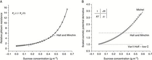
(A) Relative phloem resistance / as a function of sucrose concentration. Open circles represent the values based on viscosity data from the CRC Handbook of Chemistry and Physics (2011), and the solid line represents the fitted rational function used in this study. (B) Scaled osmotic potential derivative, . Open circles represent values calculated according to Michel (Michel, 1972; Thompson and Holbrook, 2003a). The derivative is shown rather than because it is the derivative that enters the phloem transport eqn (4). Because of the complexity of the analytical expression for the derivative, a simpler fitted polynomial function was used in this paper (line graph). For comparison, the approximate linear expressions (corresponding to eqns (6) and (7)) used by Hall and Minchin (2013) are shown by dashed lines in both (A) and (B). The value of , corresponding to the Van’t Hoff approximation for osmotic potential used in many models is also shown, by a dotted line (B).
for sucrose solution, where , , and are parameters. When the range of variations in the system is known a priori, the values of the parameters in eqns (6) and (7) can be optimized for the best fit in this range (see Fig. 2 in Hall and Minchin, 2013). However, in the context of modelling transport in a growing plant, global linear approximations are not suitable because distribution and variation within the system are not known a priori; they change with time and tree size. In this paper we used non-linear expressions for and based on the literature (see Fig. 1 for details, which also shows the linear approximations, eqns (6) and (7)). The equations for transport in internodes derived in this section are used in an iterative computational procedure solving transport in a plant structure, which estimates and for the current step using the obtained in a previous step.
First consider the case where the effect of xylem water potential gradient is small compared with the osmotic potential gradient in the phloem:
Neglecting this term in eqn (4) gives a closed-form non-linear equation for consistent with the Münch hypothesis:
where is phloem resistance to carbohydrate mass flux per unit length of phloem vasculature. Seleznyova and Hanan (2017) have shown that for the range of the internode length in plants, variations of and within an individual internode can be neglected, hence we used ,, where is carbohydrate concentration in the middle of this internode. Using this approximation, eqn (9) can be transformed to a linear form
by introducing a new variable termed ‘carbon potential’ (Seleznyova and Hanan, 2017):
Integration of eqn (10) gives the distribution of carbon potential in the internode (Fig. 2),
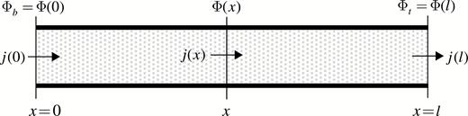
Stylized representation of an internode phloem conduit. and are the carbon potentials at the bottom and top ends of an internode, respectively. In the absence of sources/sinks, the axial mass flux of the carbohydrate,, conserves along the internode. In the presence of sources/sinks, can be calculated using the mass conservation equation; see eqn (16) and the paragraph preceding the equation.
where is the total internode resistance to the carbohydrate flux. Carbon potential is a linear function of . Carbohydrate concentration distribution in the internode can be obtained using eqn (11), .
In the case of known non-zero water potential gradient , the equation for becomes
The carbon potential distribution can be calculated by integrating eqn (13),
where
is the internode ‘xylem pull’, a term representing the effect of xylem water potential difference on phloem transport (subscripts and correspond to the bottom and the top of the internode). To determine the effects of approximations made in the above derivations on the solutions for phloem/xylem transport, L-system outputs were compared with exact analytical solutions by Hall and Minchin (2013) and with numerical solutions, obtained by Thompson and Holbrook (2003a).
While internodes in plants serve as elements of the transport system, they also have associated sinks and sources, which are distributed, e.g. primary and secondary growth, maintenance and reserves. In the original version of C-TRAM, the internode sinks/sources were considered discrete and localized at the top of the internode (Allen et al., 2005; Prusinkiewicz et al., 2007a; Cieslak et al., 2011a). This could lead to significant errors in the L-system outputs, depending on other system variables and parameters (Seleznyova and Hanan, 2017). It is possible to incorporate distributed sinks and sources into the system without major changes in the computational procedure. Consider a case where a sink is homogeneously distributed within an internode of length . For simplicity, in this derivation we assume ; however, it can be generalised for . For a quasi-stationary flow, the amount of soluble carbohydrate within a volume remains the same and the difference between the axial fluxes of carbohydrate in and out of the volume equals sink uptake . Hence the axial flux through an internode cross-section at point (Fig. 2) is given by
Note that along the internode decreases because of the carbon uptake by the distributed sink and increases in the case of a distributed source. Integration of eqn (10) using eqn (16) for gives the distribution of carbon potential:
If there is more than one distributed sink/source in the internode, eqn (17) is still valid if is a sum of the corresponding sink/source fluxes.
Mathematical model: sinks and sources
The Michaelis–Menten function (Thornley and Johnson, 1990; Minchin et al., 1993) was used for modelling carbohydrate influx into sinks,
where and are the sink attributes (examples of source functions can be found in Cieslak et al., 2011a). Because in the current model the carbohydrate distribution is represented by the carbon potential rather than the carbohydrate concentration, the sink/source functions have to be expressed in terms of by the substitution . The computational procedure at a plant level requires linearization of the source/sink functions at each time step. In the electric circuit analogy of C-TRAM, each linearized source/sink is represented by a linear electric circuit with an internal resistance and electromotive force (Prusinkiewicz et al., 2007a). In this paper, we chose to represent the source/sink functions by linear approximations in a standard form, namely
where the parameters are calculated as follows:
using the current value of the carbohydrate potential in the source/sink vicinity. This simple form is equivalent to the first two terms of the Taylor series for and it is well suited for computations at a plant level. Note that linearization parameters cannot be interpreted as source/sink attributes because they depend not only on the source/sink itself, but also on the current value of the carbohydrate potential in the sink/source vicinity. The set of parameters could be different when linearization is performed for a different value of even if the source/sink itself has not changed ( and remaining the same).
Computational procedure
The models are specified using the L+C plant modelling language, which incorporates L-systems concepts into C++ programs (Karwowski and Prusinkiewicz, 2003; Prusinkiewicz et al., 2007b). In L-systems, a specific module composed of an identifier plus associated parameters represents each plant component, while production rules specify transformations of the modules making up the plant in parallel over time. In order to include different aspects of physiological functionality, we use the aspect-oriented approach, in which each plant component is specified not as one module but as a sequence of modules (a multi-module), with each module representing a different aspect of the component’s function; for a detailed description of this approach, notations and examples see Cieslak et al. (2011b). In our model, for example, the modules associated with an internode (or a stem section) corresponding to architectural development, carbohydrate and water transport are represented by the following declarations in L+C:
/* Internode with attributes:
node,age,order,developmental age,length,radius */
module Internode(float,float,float,float,float,float);
module S(SegmentData);
module Hd(HydraulicData);
Production rules are specified independently for the water transport and carbon allocation aspects; this is implemented using the L+C Group construct; the flow of computational phases is shown in Fig. 3. In a production rule, the modules to be matched are specified in the predecessor, at the beginning of the rule. Names are given for all the parameters, so that current values for the module under consideration can be accessed. Aspect weaving or communication between aspects was made possible through the use of pseudo-L-systems in the development aspect, where the strict predecessor of a production rule was specified as a multi-module. This allowed all of the modules representing the various aspects of a component to be produced as required, and to share information as needed. In particular, interaction between the water and carbohydrate transport was taken into account by calculating the xylem pull term and the Münch counter-flow term for the current time step using the solutions obtained in the previous time step (see the following sections). This approximate method allowed decoupling of the (current step) equations for the carbohydrate and water fluxes in the internodes and solving them by applying independent production rules.
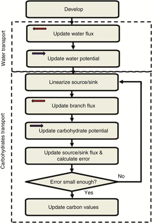
Phases of the simulation, each performed by an L-system derivation step. Arrows in the phase boxes indicate the direction that the L-system string is scanned. In the Develop phase the plant structure and the multi-module for each organ is updated. This includes the information exchange between the water and carbohydrate transport modules for calculation of the Münch counter-flow and the xylem pull terms. Due to the simple boundary conditions for water transport in this model, only two derivation steps were required to calculate water flux and water potential in the system. The carbohydrate transport computation required several phases to complete, because the source/sink fluxes are represented by non-linear functions of the carbon potential.
Water transport computational phase
The water transport aspect was added to the L-kiwi model by Dzierzon and Seleznyova (2013). Here we use a simplified version suited for fixed boundary conditions for water fluxes, which required only two computational phases (Fig. 3).
For the water transport aspect, plant organs are represented by a data structure as follows:
struct HydraulicData
{
double rs; /* xylem resistance of the internode */
double flow; /* total water flux jw through the internode */
double pot; /* water potential at top of internode */
double mcf; /* Münch counter flow,jMCF */
};
Note that we used total water flux rather than xylem flux as a system variable, firstly because it conserves along the internode and secondly because the boundary conditions in plants (leaf transpiration and root water uptake) are usually expressed in . During the daytime the difference between the two variables can be neglected.
Carbohydrate transport aspect computational phases
The essence of C-TRAM is to compute the quasi-stationary concentration and flow of carbohydrate throughout the plant using an iterative procedure based on the Newton–Raphson method (Press et al., 1992). We used the same idea but the actual implementation is different because of the choice of system variables. Rather than phloem flux and voltage variables we used mass carbohydrate flux and carbon potential (eqn (11)). We also used source/sink linearization parameters , (eqn (20)) rather than internal resistance and electromotive force . The phases of simulation are shown in Fig. 3.
Each component of the structure has an associated set of parameters called SegmentData structure, similar to that in Prusinkiewicz et al. (2007a), e.g.
struct SegmentData
{
LinearData sink_source; /* linear approximation parameters */
float xp; /* xylem pull */
float r; /* internode resistance to carbohydrate flux */
LinearData branch_flux; /* branch flux function parameters */
float j; /* carbohydrate flux into the source/sink */
float cpt; /* carbohydrate potential at the top node Φt*/
float cpb; /* carbohydrate potential at the bottom node Φb */
float err; /* current difference between iterations */
float C; /* carbohydrate in segment (structural or reserves) */
void Update_Branch_Flux(); /* updates branch_flux function parameters */
};
Here, LinearData sink_source relates to the sink/source associated with an internode (e.g. primary growth); the linear approximations of the sink/source functions are calculated during the Linearize computational phase. xp and r are updated in the Develop phase. LinearData branch_flux is carbohydrate flux through the bottom node of an internode expressed as a linear function of the node carbon potential (just like a linearized source/sink function, (19)); this flux can be interpreted as the flux into the branch starting with this internode. The calculation of the branch flux for internodes with discrete sinks and sources attached to the top is illustrated in Fig. 4. In the model code, this calculation is performed by Update_Branch_Flux();. When there are two (or more) terminal elements attached to the top of the internode, they are first represented as one linear element and then the branch flux function of the internode is calculated. During the UpdateBranchFlux computational phase the L-system string is scanned from right to left and the branch_flux function for each node is calculated. Boundary conditions (if any) are applied at the bottom node before performing the phase UpdateCarbonPotential starting from the bottom node of the plant. These calculations are just as straightforward as the ones illustrated in Fig. 4. Figure 5 illustrates calculations of the branch function for the case when the internode source/sink is homogeneously distributed along the internode. The calculations are based on eqns (16) and (17) and for simplicity assume . General equations for are also easy to obtain. The model code implementing the computational procedures described above is presented in Supplementary Data Model S1, Model S2 and Model S3.
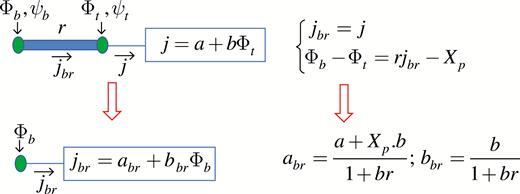
Calculation of the branch function for an internode with a terminal element attached to the top node. The purpose is to express as a linear function of the carbon potential at the bottom of the internode . In the absence of sinks and sources in the internode, the carbohydrate fluxes through the top and bottom ends of the internode are the same. The carbon potential increment can be obtained from eqn (14) by setting . The branch function parameters are determined from the equations at the top of the figure using elementary algebra.
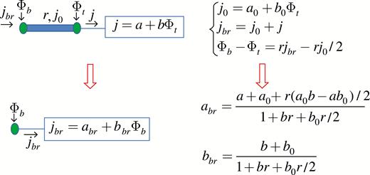
Calculation of the branch function for an internode with a distributed source/sink and a terminal element attached to the top node. Starting equations are obtained from eqns (16) and (17) by setting . The branch function parameters are determined from the equations at the top of the figure using elementary algebra.
TRANSPORT CASE STUDIES
The model presented here is based on a number of approximations. To test the validity of the approximations and evaluate their effects on model outputs we have carried out a number of case studies for simple systems including comparisons with previous exact analytical (Hall and Minchin, 2013) and/or numerical (Thompson and Holbrook, 2003a) studies.
Piece-wise analytical/L-system model solutions explained
To test the validity of piece-wise analytical/L-system solutions, the model output was compared with the exact solution for phloem flux in a cylinder obtained by Hall and Minchin (2013) using the Lambert W function. In this comparison, we assumed linear dependence of the local phloem resistance and osmotic potential on the carbohydrate concentration (eqns (5) and (6) and Fig. 1), because the solution of Hall and Minchin (2013) is available only for this case. The boundary problem was to find a carbohydrate concentration distribution along the cylinder necessary to maintain a stationary flux of carbohydrate , given the carbohydrate concentration at the bottom of the cylinder . Hall and Minchin (2013) used substitutions and analytical transformations of the eqns (1a, b), (2a, b) and (3) to reduce the problem to an equation for the Lambert W function for the whole cylinder (see Appendix 1 in Hall and Minchin, 2013). This special function is not implemented as a standard C++ function, hence we adapted the code provided by A. Hall (Plant & Food Research, New Zealand) for its calculation. In our model, the same problem was solved by dividing the cylinder into sections (internodes), using approximate analytical solutions within each internode and then connecting the solutions together by adjusting node values of the carbon potential using an iterative procedure. The nature of the approximations was that the values of the resistance to carbohydrate flux and the gradient of the osmotic potential in an internode for the current iteration were determined using the values of the carbohydrate concentration in the middle of the internode obtained during the previous iteration. Hence the variations of the osmotic potential gradient and the phloem resistance within an internode were neglected; this allowed derivation of simple solutions (eqns (14) and (17)) well suited for the downstream calculations of the branch functions (Fig. 4). It was shown previously that for typical values of internode length in plants, the effects of the above approximations are negligibly small (Fig. 3 in Seleznyova and Hanan, 2017). In the case study presented in Fig. 6, the system parameters and boundary conditions were chosen to produce a non-linear distribution with a significant range of variation to demonstrate the robustness for the current model for the case . Note that depending on the cylinder length, phloem resistance and the values of boundary conditions, the stationary solution does not always exist.
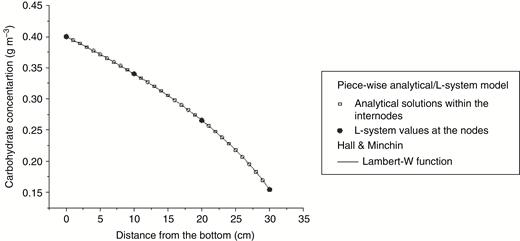
Piece-wise analytical/L-system model solution versus exact Lambert W function solution for carbohydrate concentration distribution within a cylinder obtained by Hall and Minchin (2013). The continuous analytical solution within the internodes is shown for a discrete set of x values for the purpose of comparison with the exact solution shown by the line graph.
Effect of xylem water potential gradient on phloem transport
In our model, the effect of the xylem water potential gradient on phloem transport is taken into account by introducing the xylem pull term, . For each time step, this term is calculated using eqn (15) with the pertinent variables and parameter values obtained during the previous step. In this case study, we investigated the robustness of proposed methods for phloem/xylem coupling by comparing the model solutions with the exact solutions of Hall and Minchin (2013) for the same system. Figure 7 shows excellent agreement between the two. It demonstrates that non-zero water potential gradient in the xylem affects the carbohydrate concentration difference required to maintain stationary carbohydrate flux. It can be higher or lower depending on the sign of the gradient. The model output for the water potential distribution in the system is also in excellent agreement with the results of Hall and Minchin (2013) for both daytime and night-time scenarios (data not shown).
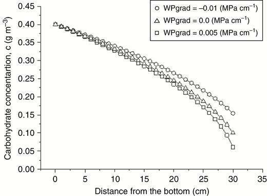
L-system model solutions (open symbols) versus the corresponding exact Lambert W function solutions (line graphs) obtained by Hall and Minchin (2013) for carbohydrate concentration distribution within a cylinder, taking into account the effects of xylem water potential gradient on phloem transport.
Effects of non-linearity of and on phloem transport
Thompson and Holbrook (2003a) obtained non-stationary numerical solutions for phloem transport in an idealized 5-m sieve tube, taking into account non-linearity of and and assuming that xylem water potential is zero along the pathway. The sieve tube was divided into a loading zone (source), a transport zone and an unloading zone (sink) (see Fig. 1 in Thompson and Holbrook, 2003a). The system evolution was simulated for a period of 24 h and by the end of this period the system approximately achieved a steady state. Hall and Minchin (2013) used the transport zone part of this steady-state solution to compare with the results of their analytical model. Using the same system configuration and boundary conditions for concentration and flux of carbohydrate ( and ), we conducted a number of case studies with different approximations for and . Initially we experienced convergence problems associated with the large size of the system; our estimated initial values of the system variables (which are required for L-system initiation) were probably not close enough to the solutions for the stationary phloem flux. This difficulty was resolved by starting with a shorter cylinder and then gradually ‘growing’ it to the required size by adding internode sections and computing the transport solutions at each step. The model outputs for the carbohydrate concentration distribution in the tube are presented in Fig. 8A together with the numerical solutions of Thompson and Holbrook (2003a, (eqn (6)) gives a relativity good agreement between the L-system results (which in this case are identical with the analytical solutions of Hall and Minchin (2013)) and the numerical solutions of Thompson and Holbrook (2003a). However, an a priori knowledge of the solution was required to optimize the linear approximation parameters. Using a non-linear function for based on the data (Fig. 1A) improves the agreement between the two models; however, the curvature of and is still not well represented. Only when both and are represented by non-linear functions is an excellent agreement between the two models achieved. This is not surprising because it is the derivate and not the function itself that enters the transport equation (eqn (4)). Even though a linear approximation for (eqn (6)) as used in Hall and Minchin (2013) (and Fig. 2a therein) is very good within the range, the corresponding approximation for the derivative can differ considerably from the actual derivative, as shown in Fig. 1B. These case studies highlight the importance of the choice of representation for . Figure 8B presents the phloem flux and the lateral water flux along the tube. The former was calculated from eqn (2b) and the latter was calculated by numerical differentiation of . This is based on the relationship
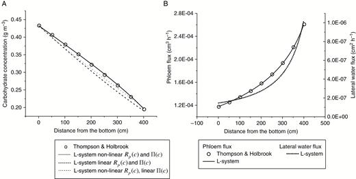
Stationary transport in a single sieve tube. The results of Thomson and Holbrook (2003a) are shown by open circles and results of L-system simulations are shown by line graphs. (A) Effects of the choice of approximations for the phloem resistance, and osmotic potential, on the simulated carbohydrate potential distribution in the tube. See Fig. 1 for the corresponding approximations. (B) Simulated phloem flux and the lateral water flux in the tube.
which is valid for the case of water potential equilibrium between phloem and xylem (Hall and Minchin, 2013). Figure 8B shows that, in the case of stationary flow, the volumetric phloem flux along the tube, , increases because of the influx of the water from xylem, . This influx dilutes the carbohydrate solution in the tube, thus maintaining the carbohydrate concentration gradient along the tube. For the case of negligible lateral resistance between phloem and xylem, this is the only possible mechanism consistent with the model formulation and, in particular with eqn (1a, b), the conservation of carbohydrate flux, based on the assumption that the membrane between phloem and xylem is impermeable to the carbohydrate molecules.
Testing solutions for systems with distributed sinks
No previous solutions were available for systems with distributed internode sources/sinks. For this case, we compared solutions for distributed systems with solutions for corresponding systems with discretized sinks. In the original version of C-TRAM, sources and sinks associated with internodes, such as structural growth, maintenance and reserves, are represented by discrete elements attached at the top node. Seleznyova and Hanan (2017) conducted a case study of the effects of source/sink discretization by simulating phloem transport in a linear conduit for different values of internode length. They demonstrated that discretization of internode sources and sinks can significantly affect the L-system solutions (Fig. 3A in Seleznyova and Hanan, 2017). In the current study, we simulated phloem transport in the same system with the difference that the internode sinks/sources were considered to be distributed homogeneously. It was demonstrated that the transport solutions for systems with the distributed sinks/sources are not as sensitive to the choice of internode length as they are to the corresponding solutions for systems with discretized sinks/sources. In fact, for the system in question the distributed system solutions for the internode values between 1 and 15 cm were practically indistinguishable (results not shown). As expected, the solutions for the system with discretized sinks/sources were converging to the solutions for a distributed system as the space resolution of the system increased (internode length decreased) and for the internode length of 1 cm the solutions for the two cases were very close. The possible consequences of the choice of internode length in the case of distributed systems are associated with the approximations of the phloem resistance of osmotic potential, which were set to their values in the middles of the internodes. The conducted case studies confirmed the validity of these approximations for the range of internode length values observed in plants.
Effects of distributed sinks/sources on phloem transport
In order to examine the possible effects of sink activity associated with the trunk on carbohydrate transport, we upgraded the model to include possible distributed sinks along the transport system. We considered three scenarios where 0 % (case 1), 33 % (case 2) and 50 % (case 3) of the carbohydrate flux produced by the canopy were taken up by the sinks distributed in the trunk and the rest were taken up by the roots (see Fig. 9 for the model outputs). Interestingly, the presence of distributed sinks has a much stronger effect on the distributions of and than on carbohydrate concentration. A stronger effect on can be explained from eqn (2b) and the fact that in the presence of sinks decreases down the trunk. Sink presence affected not only the values of but also its variation. In this study the variation was minimal in case 2 when the trunk sinks took up approximately one-third of the carbohydrate produced by the canopy (Fig. 9C). The lateral flux of water from xylem into phloem was also very sensitive to the presence of sinks in the transport system (Fig. 9D). It was positive in the absence of sinks and negative when half of the carbohydrate produced by the canopy was taken up by distributed sinks. The smallest variation of the lateral flux was achieved in case 2 when approximately one-third of the carbohydrate produced was taken up by the sinks in the transport system. In this case the lateral flux has changed its direction, being positive at the top of the tree and negative at the bottom. As explained above, the lateral flux regulates the carbohydrate concentration gradient required for the maintenance of the stationary flow. In the presence of distributed sinks, the sink activity has also contributed to the dilution of the phloem flux along the transport system and hence affected the lateral water flux.
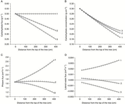
Effects of distributed sink on phloem transport in a tree trunk model. Case 1, no distributed sink in the system; case 2, ; case 3, . Carbohydrate flux in the system (A) and the corresponding carbohydrate distribution (B), phloem flux (C) and lateral flux (D). Positive and negative values of correspond to influx and outflux of water, respectively.
Note that because of the non-linearity of the equations with respect to carbohydrate concentration, the solutions presented here are not scalable with respect to the boundary conditions and, although the mechanisms explained by the example presented here are valid in general, the quantitative solutions for each individual boundary problem should be obtained individually.
DISCUSSION
Transport of water and carbohydrates is essential for plant survival at an individual and a population level (Nikinmaa et al., 2014; Knoblauch and Peters, 2016; Savage et al., 2016). The growth and development of individual trees results from complex interaction between carbohydrate sinks and sources mediated by the tree transport system (Allen et al., 2005). Nikinmaa et al. (2014) presented a comprehensive model linking the leaf gas exchange phloem/xylem transport and source activity within an 8-year-old Scots pine tree. Their analysis of model behaviour suggested strong linkage between the current tree structure, gas exchange rate and the potential for new growth. However, because their model was developed for a static structure, it was not capable of simulating dynamic interactions between these aspects in the course of tree development and growth. The current paper presents a mechanistic model of quasi-stationary phloem/xylem transport in a developing tree structure. This was achieved by a combination of analytical and computational methods using an L-system-based modelling platform for model implementation. Physical processes associated with transport are governed by differential equations. For numerical solutions, the system is usually discretized and the equations are transformed to a finite-difference form (as, for example, in Nikinmaa et al., 2014). In this case, the model resolution depends on the temporal/spatial resolution of the system and computations at higher resolutions require more time (see, for example, the discussion of these issues in Thompson and Holbrook, 2003a) with respect to the example presented in Fig. 8. In our model, the plant was represented at a metamer level with the internodes represented by conduit elements and the lateral organs represented by sources and sinks. Our approach is based on the consideration that, although internode length in most plants could be too large as a unit of spatial discretization by the standards of discrete numerical methods, it is small enough for making some simplifying approximations and solving the differential transport equations analytically for individual internodes. The choice of system variables, and in particular the carbon potential (eqn (11)) variable first introduced by Seleznyova and Hanan (2017), was essential to extending the solutions to a plant level. This allowed solutions of the transport equations within an internode to be expressed as linear functions of the boundary conditions at the bottom node. Linearity of these solutions was critical for computing solutions for carbon potential and carbohydrate concentration at a plant level. The developed approach is particularly suited for solving transport equations in systems with distributed sinks and sources, such as internode maintenance, secondary growth and reserves. The extensions of the continuous analytical solutions within the internodes and of the rules for calculation of carbohydrate fluxes throughout the plant were very straightforward. Interactions between xylem and phloem transport were taken into account using an aspect-oriented approach (Cieslak et al., 2011b). At each developmental step of the model, first the interaction terms, xylem pull and the Münch counter-flow were calculated and passed to the corresponding data structures in water and carbohydrate aspects. The water and carbohydrate transport solutions at a plant level were then calculated taking into account these terms.
Our methods are based on a number of approximations made in both analytical and computational parts of the problem. In the former, the phloem resistance and the osmotic potential gradient were assumed constant within each internode and were approximated by the carbohydrate concentration at the centre of the internode. This considerably simplified the solutions at an internode level and made them suitable for use in calculations at a whole-plant level. Our expectation was that approximations at the internode level should not prevent taking into account more realistic representations for phloem resistance and osmotic potential at a whole-plant level. To test this, we simulated transport in simple linear systems where solutions obtained by other methods were available. It followed from the analysis of the transport equations that the effects of the above approximations should be stronger for systems with higher values of the carbohydrate concentration gradients. Hence the choice of boundary conditions and model parameters for the first case study was made to achieve such a scenario. We chose the same linear approximations for phloem resistance and osmotic potential as in Hall and Minchin (2013) so as to be able to test our model solutions against their analytical solutions in terms of the Lambert W function. This comparison demonstrated excellent model performance, even for extreme gradients of the carbohydrate concentration gradients (Figs 6 and 7). Comparison of our results in the case of non-linear phloem resistance and osmotic potential with those of Thompson and Holbrook (2003a) supports the validity of our approximation for these variables at a metamer level. Our results confirm the conclusions of Hall and Minchin (2013) about the importance of adequate representation of these variables. When the Van’t Hoff relation is used for osmotic potential, the carbohydrate potential gradient necessary to drive the phloem flux is hugely overestimated (see Fig. 3 in Hall and Minchin, 2013), yet some papers on phloem transport in trees use this relationship to draw general conclusions (Thompson and Holbrook, 2003b; Jensen et al., 2011). Another aspect that is often overlooked is the importance of sinks and sources distributed along the transport pathway between the primary sources of tree crown and the root sink. However, it is documented that the annual trunk dry weight increment of a tree can be higher than that of the root system (van Hooijdonk et al., 2016), which also implies the higher maintenance cost of the trunk and a higher reserve accumulation capacity. Hence the trunk sink requires considerable influx of carbohydrate from the transport system. On the other hand, the large amount of reserves stored in the tree trunk acts as buffer of the carbohydrate supply when the influx from the primary sources is limited (e.g. early spring, canopy damage). Our study of the systems with sinks distributed along the transport pathway demonstrated a strong effect of the distributed sinks on the phloem flux. This result is in agreement with the conclusions of Nikinmaa et al. (2014), who reported that the model behaviour was very sensitive to the formulation of sink activity in the internodes. Our study has emphasized the importance of clearly distinguishing between the volumetric phloem flux and the mass carbohydrate flux when quantifying phloem transport. Although these two variables are related (eqn (2b)), the relationship does not conserve along the transport system and it is affected by the lateral water exchange between phloem and xylem and the presence of sinks and sources. This study confirmed a previous result that in the absence of the sinks/sources when the carbohydrate mass flux conserves along the pathway, the phloem flux increases (Fig. 8B), as discussed by Thompson and Holbrook (2003a) in Appendix 1 of their paper. The current study has particularly emphasized the sensitivity of the lateral water flux along the pathway to the presence of distributed sinks/sources. In particular, in the transport-only pathway the lateral flux of the water increases to maintain the carbohydrate concentration gradient and the stationary phloem flux (Fig. 9D, case 1). This conclusion contradicts the schematic of the lateral flux presented in Fig. 1 of Thompson and Holbrook (2003a), which shows a change of sign of the lateral water flux along the pathway. Based on our study, in the case of the stationary transport, the lateral flux can change sign only in the presence of sinks/sources (see for example Fig. 9D, case 2). One limitation of this work is the assumption of water potential equilibrium between phloem and xylem (high Münch number). This assumption is supported by the conclusion of Thompson and Holbrook (2003b); see also Table 2 in Jensen et al. (2011) showing high values of the Münch number for trees. In the future the methods will be extended to systems with finite resistance between phloem and xylem.
In conclusion, this paper presents the development and testing of novel methods for mechanistic modelling of stationary phloem/xylem transport in developing plants. The critical difference from previous work is the application of analytical methods at a metamer (internode) level, which allows continuous solutions for the system variables at whole-tree/vine level to be obtained and increases the model’s spatial resolution without increasing computational time. The methods are particularly suited for systems with distributed sinks/sources along the transport pathways. Possible applications of this work are fine-scale modelling of carbohydrate distribution within plants, the modelling of leakage–retrieval processes along the transport pathways, and the development of growth-unit-scale models with distributed sink/sources.
SUPPLEMENTARY DATA
Supplementary data are available online at www.aob.oxfordjournals.org and consist of the following. Model S1: coupled phloem xylem model test. Model S2: coupled phloem xylem transport model. Model S3: distributed system transport model. The models run on L-studio ATE 4.4.1-2976 (13 July 2016), downloadable from algorithmicbotany.org/virtual_laboratory.
ACKNOWLEGEMENTS
We thank Dr H. Dzierzon for implementation of the original code for water transport and Dr A. Hall for useful discussions and comments on the first draft of this paper. This project was funded by The Discovery Science Fund, Plant & Food Research, New Zealand.
LITERATURE CITED
CRC Handbook of Chemistry and Physics. 2011. In: ed Haynes WM, ed. 92nd edition. Boca Raton, FL: CRC Press, 5–145.
