Plant growth and respiration re-visited: maintenance respiration defined – it is an emergent property of, not a separate process within, the system – and why the respiration : photosynthesis ratio is conservative Open Access

Abstract

INTRODUCTION

There continues to be considerable discussion of respiration. This is focused partly on how to handle maintenance respiration (MR) when working within the ‘growth respiration/maintenance respiration paradigm’ (GMRP) (Amthor, 2000) and partly on the ratio (r) of respiration (R) to gross photosynthesis (P_g) in plant ecosystems, defined as r_R:Pg. There is concern as to whether r_R:Pg is constant or variable. The topic is important in addressing some climate change issues, such as short-term and long-term contributions of plant ecosystems to carbon (C) sequestration. On one hand are simplifying and perhaps optimistic holists, who would like to assume that r_R:Pg is approximately constant over a range of species and conditions (e.g. Gifford, 2003). This might permit construction of simple ecosystem models applicable to climate problems. A recent example of this is Van Oijen et al. (2010), who, working within GMRP, with some assumptions, demonstrate that a more or less constant value of the ratio is to be expected, partly as a result of conservation of matter (stoichiometry). On the other are reductionists who might also consider themselves as realists. The latter, to which group I mostly adhere, make efforts to understand the detailed mechanisms of respiration which cause r_R:Pg to fall below unity and, possibly, be rather variable (Cannell and Thornley, 2000; Thornley and Cannell, 2000). Amthor (2000) gives an excellent review of plant respiration, supplying a valuable historical perspective and also the current state of the art – there have been no substantive advances in the past decade.

Mainteneance respiration is often considered to be a distinct portion of respiration, but it has long been regarded sceptically. Wohl and James (1942), remarked that ‘It is a facile assumption that the energy change revealed by the continuous liberation of heat from mature tissues which are neither doing external work nor synthesizing appreciably, is a measure of the energy of maintenance. The assumption will not stand closer inspection …’.

The construction and analysis of simple models can sometimes be employed to illuminate important problems; this is what is attempted below. A simple model without a maintenance component is described. Solutions are obtained, focusing on two important phases in the growth dynamics: exponential growth and the steady state. The first phase, exponential growth, is transient, but it often lasts sufficiently long to be characterizable, and it is amenable to experimentation. The second phase, the steady state, is important because many plant ecosystems may be approximately in a steady state, although it can be less accessible to experimentation.

We define the specific MR rate (ρ_m; d⁻¹) as being the specific respiration rate when the growth rate is zero, i.e. when the status quo is maintained. The growth rate can be zero in two cases: when the plant is in the exponential growth (eg) phase but is growing at zero rate; and when the plant is in the steady state (ss) (its mass has reached an asymptote). In both cases, the same expression is obtained for the specific MR rate, depending on three parameters of the model (Fig. 1). This permits a re-parameterization of the model, which can, with assumptions, be simplified to a form perhaps more acceptable to the holists.

Fig. 1.

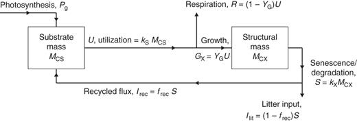
Plant growth model for respiration. The two state variables are substrate mass, M_CS, and structural mass, M_CX. There are four key parameters: Y_G, growth efficiency – fraction of substrate C utilized for growth which appears in structure – the remaining fraction (1 – Y_G) is respired; f_rec, fraction of senescing/degrading structural C recycled to substrate, the remainder becoming litter; k_S, rate constant for substrate utilization; and k_X senescence rate constant.

Open in new tabDownload slide

Current understanding of plant respiration was given impetus and direction by the findings of McCree (1970), and his famous equation:

(1)

where R is 24 h respiration (kg CO₂ m⁻² d⁻¹), P is daily gross photosynthesis (kg CO₂ m⁻² d⁻¹), W is plant mass (kg CO₂ equivalents), k is a constant (dimensionless), and c is has units of d⁻¹. McCree applied a 12 h light period during a 24 h day. Details of how R and P are obtained from the measurements are given by McCree (1970), a procedure which could be affected by daylength. McCree's estimate of the parameters was k = 0·25 and c = 0·015 d⁻¹. Dividing through by dry mass W gives

(2)

This equation relates a specific 24 h respiration rate to a specific daily gross photosynthetic rate. The simplicity and intuitiveness of these equations has contributed greatly to the appeal of the GMRP paradigm, with c being interpreted as a maintenance coefficient.

The situation here may be compared with micro-organisms in a chemostat (Pirt, 1965), where it is possible, in a true steady state without diurnality, to measure directly the gross rate of supply of substrate, respiration rate and also growth rate. This leads to a similar equation.

The meaning of eqns (1) and (2) has been much discussed over the years (Amthor, 2000). A common interpretation is that respiration is viewed as having two components: one results from growth of the organism [growth respiration (GR)]; the other (MR) is attributed to the organism maintaining its status quo (Pirt, 1965; Thornley, 1970).

Two objections can be raised against GMRP. The first is on scientific grounds: the biochemical and other processes occurring in a growing organism are qualitatively the same as those which occur in an organism which is maintaining the status quo. This especially applies to the metabolic processes which give rise to respiration and yield ATP and reducing power, but also those anabolic processes which are synthesizing compounds which in some cases are replacing compounds that have recently been catabolized. In general, there is not a distinct set of processes which can be said to belong to ‘maintenance’, and another set which belongs to ‘growth’, although catabolic processes (such as protein breakdown) may lead to a growth-associated process (protein synthesis) maintaining the status quo of the plant and giving a respiratory flux which can be dubbed maintenance.

The second objection is a practical matter: many authors have used the paradigm when constructing models of plant growth, crop growth and plant ecosystems. Again and again unacceptable behaviour of the model has occurred, and the maintenance component has to be arbitrarily ‘fixed’. For example, de Wit et al. (1970, p. 61) remarked ‘Simulation of this viewpoint leads to inconsistent results. If it is assumed that the respiration per unit plant material is low, it appears that yield levels which are observed in the field may be obtained, but then simulated respiration rates under controlled conditions are far too small. If it is assumed that respiration per unit of plant material is higher, simulated respiration rates under controlled conditions may be in the observed range, but then simulated ceiling yields in the field are far too small.’ Loomis (1970, p. 140, 141) states ‘The McCree equation R = kP + cW summarizes well certain data … but it would be a mistake to assume it holds a priori for other situations, …’, and ‘The big difficulty is, of course, in accounting for ‘maintenance’ respiration …’. The impasse is resolved (typically) by making the maintenance coefficient variable, e.g. Seginer (2003) assumes that the maintenance coefficient depends asymptotically on plant structural mass. Van Oijen et al. (2010) assume that MR equals GR, an assumption tantamount to jettisoning GMRP in favour of a growth-only respiration model. Others assume that the MR rate coefficient depends on the availability of substrates (e.g. Thornley, 1998, p. 38), as in the growth process. The problems revolve around issues such as: a common substrate (carbohydrate) is used for both growth and maintenance; priorities (more explicitly, utilization rate constants) have to be assigned between growth and maintenance; and these priorities need to change according to substrate supply and utilization (which determine substrate fraction). There is no straightforward way of dealing with growth and maintenance separately because the pools and anabolic processes are the same for both growth and maintenance. Many modellers do not like to represent substrates because their representation is perceived to be difficult (which it can be), although consideration of the differences between sub-arctic and semi-tropical plant ecosystems, and the diurnality of many plant variables including substrate pools might suggest that their representation is essential for realism.

Here a two-state variable model (structure and substrate; Warren Wilson, 1967) is described. ‘Substrate’ includes storage (easily remobilizable) components. The model is a simplification and extension of a model proposed some years ago (Thornley, 1977; see also Loehle, 1982, who expanded on the 1977 model and provided a reconciliation of it with the more traditional view of respiration). The simplification is that non-degradable structure is omitted so that steady-state solutions can be derived, providing the insights that can be obtained from analytical expressions. The extension is that senescence is included, again so that steady-state solutions can be obtained. The significant processes are photosynthesis, growth with GR, senescence and recycling to the substrate pool. Respiration is an output of the growth process alone. Maintenance is not a feature. The model is simple enough (with three significant constants) to permit a thorough exploration of its properties, for both exponential growth and the steady state. My first objective is to demonstrate that its predictions are reasonably compatible with McCree's equation [our eqn (1)] (McCree, 1970), and therefore provides an alternative to the GMRP. My second objective is to define and extract a specific MR rate for a non-growing plant (which can occur in two ways). My last objective is to show that the model gives explicit expressions and acceptable and conservative predictions for the respiration:photosynthesis ratio (r_R:Pg), which for plant ecosystems is often in the range 0·4–0·5. Approximate expressions for the parameters of McCree's equation can be derived in terms of the significant parameters of the current model.

MODEL AND METHODS

The scheme is drawn in Fig. 1. Variables and parameters are listed in Table 1. The two state variables (pools) are M_CS (kg substrate C m⁻²) and M_CX (kg structural C m⁻²); these are per unit ground area. Next the fluxes in Fig. 1 are calculated, all having units of kg C m⁻² (ground) d⁻¹.

Photosynthesis, P_g

The expression used for gross photosynthesis [eqn (4)] has a long pedigree, and is parameterized with familiar quantities. It gives the correct dependencies on plant size (leaf area index), light flux density, photosynthetic efficiency and light-saturated leaf photosynthesis. These are needed because we shall be comparing our results with measured data.

First calculate the leaf area index, L_AI, from structural mass, M_CX, with

(3)

Leaf area ratio, L_AR, is a rounded value obtained from Causton and Venus (1981, p. 46, fig. 2·6a) who give a leaf area ratio of about 0·02 m² (g total mass)⁻¹. Note that L_AR is a ‘structural’ leaf area ratio, with reference to just the structural biomass C component. Therefore, it is higher than usual, which is per unit of total biomass. We assumed that 40 % of total dry mass is structural C (50 = 1000 × 0·02/0·4). It is assumed that L_AR is constant in order to make a simple analysis feasible. However, Bertin and Gary (1998) examined leaf mass per area (LMA, g m⁻²) in tomato, manipulating light, CO₂ and fruit load. They found substantial variations of incremental LMA related to source/sink status and sugar and starch content, and used their findings to modify their modelling of tomato plant growth. Such modelling requires keeping track of leaf area age distribution and increases complexity greatly (e.g. Thornley, 1998, pp. 48–49).

Gross photosynthetic rate, P_g (kg C m⁻² d⁻¹), is calculated with

(4)

P_g is, via eqn (3), a function of the structure state variable, M_CX. This equation is based on a continuous canopy of leaf area index L_AI, light flux density incident on the top of the canopy of I₀, exponential decrease in light level on descending into the canopy of exp(– L_AI), a rectangular hyperbola for leaf response to light [P_leaf = αI₀P_max/(αI₀ + P_max), kg CO₂ m⁻² (leaf) s⁻¹] with photosynthetic efficiency of α, a light-saturated photosynthetic rate of P_max at the top of the canopy which decreases as exp(–L_AI) on descending in the canopy, and black leaves with a canopy extinction coefficient of unity [see, for example, Thornley and France, 2007, pp. 297–298, equation (9·50) with k = 1 and m = 0]. The factor 86 400 s d⁻¹ converts per second units to per day; 12/44 converts mass of CO₂ to mass of C. The light flux density I₀ of 50 here is for continuous light (giving a daily light receipt of 4·32 MJ photosynthetically active radiation (PAR) m⁻² d⁻¹ or 19·9 mol PAR m⁻² d⁻¹); elsewhere a value of 100 is applied for a 12 h day, giving the same daily light receipt.

Equation (4) is used because of its simplicity and tractability. There are other better approaches available (e.g. Thornley and France, 2007, pp. 288–301; Johnson et al., 2010). Although plant growth does of course depend on the parameters in eqn (4), the key results of our analysis are independent of the parameters in eqn (4) and its precise form, as long as the equation applied to calculate gross photosynthetic rate can be linearized for low values of L_AI so that exponential growth is a possible solution.

It will be useful later when points of inflexion are calculated to have an expression of the differential of P_g with respect to M_CX, namely

(5)

This decreases exponentially with M_CX from 0·29 kg substrate C (kg structural C)⁻¹ d⁻¹ when M_CX is small (I₀ = 50) at time t = 0 (Table 1a) towards zero as structural mass M_CX (and L_AI) → ∞.

The specific instantaneous gross photosynthetic rate, π_g [kg C (kg total C)⁻¹ d⁻¹], is

(6)

Total mass M_C is given in eqns (18); see eqn (11) for substrate fraction C_S. Note that increasing C_S decreases the specific gross photosynthetic rate.

At low and high values of light flux density I₀, eqn (4) approximates to

(7)

For low values of leaf area index, L_AI [or structural mass, M_CX, eqn (3)], we write [from eqn (4)]

(8)

Parameter β has units of per day. In carbon units, it is the fraction of current structural C added per unit time via gross photosynthesis to the C substrate pool. It is a rectangular hyperbolic function of light flux density I₀. Values in the dark (I₀ = 0), at I₀ = 50 J PAR m⁻² s⁻¹ and its maximum are

(9)

At high continuous light and low L_AI, gross photosynthesis adds C equal to approx. 60 % of the current structural C to the substrate C pool per day.

The linear expression P_g = βM_CX of eqn (8) is valuable because it means that at low values of L_AI the plant grows exponentially at a proportional growth rate dependent on I₀. Later, we use the inverse of the second of eqns (8), namely

(10)

to calculate light flux density I₀ from a given value of β. Decreasing β decreases I₀.

Substrate utilization, U, respiration, R, and structural growth, G_X

Substrate ‘concentration’ or fraction, C_S [(kg substrate C) (kg structural C)⁻¹], is a useful intensive variable, defined as

(11)

Assuming that the volume of the reaction in which substrate utilization takes place is proportional to the mass of structural C, M_CX, then the rate of substrate C utilization, U (kg substrate C m⁻² d⁻¹), is (assuming linear or mass-action kinetics with rate constant, k_S)

(12)

With all defaults and in continuous light (Table 1b), this k_S value gives a substrate fraction C_S [eqn (11)] = 0·27 during the initial exponential growth phase [eqn (25)], and C_S = 0·053 at the steady state [eqn (42)]. A total of 63 % of an initial quantity of substrate is utilized within one 24 h day [exp(–k_S) = 0·37] [eqn (12)].

Utilized flux of substrate C, U, is divided between structural growth, G_X, and respiration, R (kg C m⁻² d⁻¹) (Fig. 1) [note: we are not now using McCree's units for R; see eqn (1)]:

(13)

Y_G is a fraction (0 ≤ Y_G ≤ 1) termed growth efficiency or growth yield. Y_G values can vary considerably. The value of Y_G = 0·75 is fairly typical for vegetative plant material (e.g. Thornley and Cannell, 2000; Thornley and Johnson, 2000, pp. 350–353). No respiratory flux is associated with the senescence processes in Fig. 1. Such fluxes may exist and could be linked to outputs from a litter pool or to the inputs to that pool; they are omitted so that we retain the simplicity of a single respiratory output flux.

The instantaneous specific respiration rate, ρ [kg C respired (kg total C mass)⁻¹ d⁻¹], is [cf. eqn (6)]

(14)

For total mass M_C see eqns (18). ρ increases from zero to a maximum of (1 – Y_G)k_S as C_S increases from zero to ∞.

Senescence flux S, fluxes to litter, I_lit, and recycling of substrate, I_rec

The proportional rate at which structure senesces is k_X (d⁻¹), giving a senescence flux of S (kg structural C m⁻² d⁻¹, Fig. 1) of

(15)

The fraction senescing or degrading per day is 4 %, giving a tissue lifetime of 25 d. No distinction is made between senescence and (non-pathological) degradation, and henceforth the process is referred to as senescence. More detailed plant models may distinguish between ageing and senescence, and non-age-related tissue turnover or degradation (e.g. Thornley, 1998). No respiratory flux is associated with senescence (see above). The structural C flux from senescence is divided between a fraction, f_rec, which is recycled to the substrate C pool with flux, I_rec, and the remainder, I_lit, which is input to a litter pool (Fig. 1). Thus

(16)

It is assumed that a constant 50 % of the senescing C is recycled. In general, it may be expected that this is a variable fraction depending on nutrient status (level of substrate fraction C_S) and tissue composition. Note that 0 < f_rec < 1. In a real varying environment where substrate supply moves between scarce and plentiful, it does not seem unreasonable to take f_rec = 0·5 as representing an average value.

Differential equations

By inspection of Fig. 1 and using eqns (4), (12), (13), (15) and (16), these are

(17)

Gross photosynthetic rate P_g is written as P_g (M_CX) to emphasize that P_g is a function of state variable M_CX [Fig. 1, eqns (4), (3)]. The t = 0 value of substrate fraction C_S is 5 % [eqn (11), defining M_CS(t = 0) in terms of M_CX(t = 0)]. Denote total mass by M_C (kg C m⁻²) and its rate of change by dM_C/dt (kg C m⁻² d⁻¹); therefore,

(18)

Equations (13) and (16) have been applied. Net photosynthetic rate, P_n, is defined as gross photosynthesis P_g [eqn (4)] less respiration R [eqns (13)]. These two alternative forms for net photosynthesis, namely

(19)

are used to check model formulation (stoichiometric validity) and programming.

Proportional growth rates of state variables (μ_S, μ_X) and total mass (μ)(d⁻¹) are

(20)

These are intensive variables which are constant during exponential growth.

The instantaneous ratio (r) of respiration R [eqns (13)] to gross photosynthesis P_g [eqn (4)], r_R:Pg, is

(21)

The equation for the double differential of total system C is [differentiating the third of eqns (18)]

(22)

With eqns (17) and (5), d²M_C/dt² can be written in terms of the state variables. Hence time of inflexion when d²M_C/dt² = 0 and state variable values at inflexion can be extracted numerically.

The differential eqns (17) could be non-dimensionalized [using eqn (4)], but not uniquely. This was not seen as a helpful simplification.

Exponential growth (eg)

There are two limiting cases for which analytical solutions exist. These are first exponential growth and secondly the steady state in a constant environment. In this section we examine exponential growth (eg). Exponential growth occurs at low L_AI [eqn (8)] when eqns (17) become

(23)

β(I₀) is so written to make explicit that β is a function of light flux density I₀ [eqns (8)]. Assuming constant and equal proportional growth rates μ for M_CS and M_CX [eqns (20)] and constant substrate C fraction, C_S [eqn (11)], eqns (23) become (divide through by M_CX)

(24)

These equations are solved for μ and C_S. Eliminating μ (the positive square root gives the biologically meaningful result)

(25)

Here, ‘eg’ denotes exponential growth.

Plotting exponential growth rate μ(eg) against substrate fraction C_S(eg) gives a straight line [last of eqns (25)], with zero growth occurring when

(26)

There is a minimum (non-zero) substrate fraction of 0·05333* kg substrate C (kg structural C)⁻¹ (default parameters, Table 1b) below which the plant dies [μ(eg) < 0]. Low values of the senescence rate constant k_X and high values of growth efficiency Y_G and substrate utilization rate constant k_S lead to a low value of C_S(eg; μ = 0) [see eqn (30) below].

In terms of the underlying parameters, C_S(eg) and μ(eg) become [eqns (25)]

(27)

For small values of β(I₀) [which is proportional to light flux density, I₀, eqn (8)], these are linearly proportional to β and thence I₀ [because √(1 + x) ≈ 1 + ½x for small x]. For large β, C_S(eg) and μ(eg) ≈ √β. Remember that β has an asymptotic hyperbolic dependence on light flux density I₀, with asymptote β_max depending on maximum photosynthetic rate P_max [eqns (8), (9)].

In the dark (I₀ = 0), β = 0 [eqns (8)], eqns (27) become

(27)

Assuming that k_S ≫ k_X (Table 1b), these can be approximated by

(29)

The rate of decline in the dark is least if growth yield Y_G and recycling fraction f_rec are high (approaching unity).

The plant dies if μ < 0. For β the second of eqns (27) gives an upper limit, and then eqns (10) and (9) give an upper limit of light flux density I₀, so that μ < 0 implies

(30)

[This result can be derived directly from eqns (24) (eliminate C_S; write down the condition for μ < 0).] Death of the plant depends on light flux density I₀ [eqn (8)], but the critical values of β and I₀ for positive growth are less (giving shade tolerance) for lower values of senescence rate parameter k_X, and for higher values of growth yield Y_G and recycling fraction f_rec. There is no dependence on substrate utilization rate constant k_S [eqn (12)].

At zero growth rate, the plant is just maintaining its status quo. The specific maintenance respiration rate [eqn (14)], ρ_m, is [with eqn (26)]

(31)

Values for default parameters (Table 1b) are given. There is weak dependence on utilization rate k_S [eqns (12)] as generally Y_Gk_S ≫ k_X. ρ_m does not depend on recycling fraction f_rec (Fig. 1) [but see Fig. 4B and eqns (56) – the intercept of McCree's equation does depend on the recycling fraction f_rec].

The specific respiration rate for a plant in exponential decline in the dark is [eqns (14), (28)]

(32)

For k_S ≫ k_X, this is approximately (1 – Y_G)f_reck_X = 0·005 d⁻¹ [use eqns (29)]. This quantity is sometimes assumed to be a measure of the MR rate, but it is substantially less than the specific respiration rate required to maintain the plant's status quo [eqns (31)].

The specific gross photosynthetic rate, π_g [eqns (6), (8), (13)], for exponential growth, is

(33)

For a given light level and value of β [eqn (8)], π_g decreases as the sugar level in the plant [C_S(eg), eqn (27)] increases (due perhaps to a decreasing k_S; Fig. 1, eqns (12)].

The ratio of respiration to gross photosynthesis (19) is [eqns (13), (8), then (27)]

(33)

The numerical value given is for I₀ = 50 W (PAR) m⁻² (230 µmol PAR m⁻² s⁻¹) giving β [eqn (8)] = 0·2945 d⁻¹. At zero growth rate this becomes

(35)

Here we used the second of eqns (30) with the equality to substitute for β and eqn (26) for C_S in the first line of eqns (34). The ratio at zero growth rate (maintenance) is 0·4 with default parameters (Table 1b) or 0·25 with no recycling (f_rec = 0) [see paragraph after eqns (16); also eqns (30) and following paragraph].

Steady state (ss)

In eqns (17), put the derivatives equal to zero, giving (ss denotes the steady state)

(36)

Solving for M_CS, M_CX and adding to give total mass M_C, therefore

(37)

To find the steady state, solve two equations for P_g(ss) and M_CX(ss) [from eqn (4) and the second of (37)]:

(38)

Eliminating P_g(ss) gives

(39)

This transcendental equation can be solved numerically for M_CX(ss), e.g. using the Newton–Raphson method (Thornley and France, 2007, pp. 830–831), noting that eqn (39) is easily differentiated with respect to M_CX(ss). There is a trivial solution at M_CX = 0. There is a non-zero solution only if, at small M_CX, the slope of the right side of eqn (39) is greater than that of the left side. Therefore, using eqn (8) (P_g = βM_CX),

(40)

This inequality is equivalent to eqn (30) for plant death during the exponential growth phase. With eqn (10), it is equivalent to I₀(μ > 0) >3 J (PAR) m⁻² s⁻¹ [14 × 10⁻⁶ mol (PAR) m⁻² s⁻¹] for standard parameters (Table 1b) [cf. eqn (30) and following paragraph].

Given that eqn (40) is satisfied and a non-trivial steady-state solution to eqn (39) exists for M_CX(ss) and therefore also P_g(ss) with either of eqns (38), the respiration rate R in the steady state becomes [eqns (13) and (37)]

(41)

Hence follow several important ratios for steady-state plant ecosystems [for C_S(ss), use eqn (11) and the second of eqns (36)], with parameters from Table 1b:

(42)

These are all independent of environment, here light flux density, in contrast to these quantities during exponential growth [eqns (27), (34)] where they depend on β and light flux density I₀ [eqn (8)] apart from the specific MR respiration rate, ρ_m [eqn (31)]. The last of eqns (42), for specific respiration rate in the steady state, is obtained from the first of eqns (41) and the last of eqns (37). This is identical to eqn (31) for the specific respiration rate of a plant growing exponentially at zero rate. This important general result provides a link between long-term ecosystem behaviour and short-term experimentation on young plants. The R:P_g ratio in eqns (42) has a simple interpretation with the Fig. 1 model because the denominator, 1 – x (say), can be expanded as 1 + x + x² + x³ …, giving successive cycles of substrate use and re-use.

Diurnal environment

Assume that light flux density I₀ [eqn (4)] is varied on a daily basis, with 12 h of light followed by 12 h of darkness. The analysis of the last two sections dealing with exponential growth and a steady state in a constant environment is no longer possible. However, this more realistic situation can be examined numerically, obtaining results that may be compared with measurements such as those by McCree (1970) as well as with our analytical results for continuous light.

Define fractional daylength, f_dl, by

(43)

Light flux density I₀ applied in eqn (4) to calculate photosynthesis is adjusted by dividing by fractional daylength:

(44)

The symbol ‘: = ’ means the value is replaced by. This ensures that daily light receipt is the same and makes simulations of a constant light regime and a 12 h day more comparable.

A critical issue is how, for a diurnal environment, are ‘daily gross photosynthesis’ and ‘daily respiration’ defined. These quantities, denoted by P_g,day (kg C m⁻² d⁻¹) and respiration, R_24h (kg C m⁻² d⁻¹), are calculated with [eqns (4), (13)]

(45)

Daylength is 12 h and light is applied from 0 to 12 h and darkness from 12 to 24 h. The ratio of 24 h respiration to daytime gross photosynthesis is

(46)

These quantities are calculated so that a comparison (albeit imperfect) with McCree's (1970) results can be made.

CO₂ gas exchange measurements generally give directly net photosynthesis during the day and respiration during the night. Again for comparison, and using an obvious notation, eqns (45) and (46) can be extended (including the fraction of 24 h respiration occurring during the night) [eqns (19), (13)]

(47)

Specific values of daily photosynthesis and respiration are calculated by dividing by total mass M_C [eqns (18)] at the end of each 24 h day:

(48)

An exponential growth phase still occurs, now on a daily (24 h) basis rather than an instantaneous basis; there are fluctuations in proportional growth rates during the day [eqns (20)]. The steady state becomes a 24 h equilibrium state with diurnal variation.

Re-parameterization of the model

A more traditional single-state variable plant growth equation [cf. eqns (17) with two state variables] is obtained by making a zero-pool approximation (Thornley and France, 2007) and by eliminating one parameter in favour of a synthetic (emergent) McCree-type parameter.

Specific MR rate, ρ_m (d⁻¹), is [eqns (31) or (42)]

(49)

Any of the three parameters: k_S, k_X or Y_G (Fig. 1) can be eliminated from the model in favour of ρ_m. We eliminate k_X, writing

(50)

The differential eqns (17) become

(51)

For large values of k_S, substrate content M_CS is small, and is treated as a ‘zero pool’ so that inputs = outputs, dM_CS/dt ∼ 0. Also assuming that (1 – Y_G)k_S ≫ ρ_m [eqns (13), (12), (31), (42)], the first equation becomes

(52)

Substituting for k_SM_CS from eqn (52) in the second of eqns (51), and again for large k_S [eqn (49) is used for the specific MR rate, ρ_m]:

(52)

Finally

(54)

This is a single-state variable plant growth equation. The coefficient (for k_S = 100 d⁻¹), m, is

(55)

This can be compared with the specific MR rate of ρ_m = 0·0133* d⁻¹ [eqn (31)]. It is mistaken to interpret m as the maintenance requirement. Integration of eqn (54) or of eqns (17) with k_S = 100 d⁻¹ (say) gives exactly the same time course for M_CX, so long as respiration is still defined by eqns (13).

This result depends on the assumptions in Fig. 1. The crucial assumption concerns respiration rate R [here given by eqn (13) with k_SM_CS now given by eqn (52) in the zero-pool approximation]; the rest is stoichiometry. Equation (13) is what Warren Wilson et al. (1986) call a ‘conditional’ equation which represents a scientific hypothesis. When C conservation (stoichiometry) is considered, many equations that are ‘identities’ can be written down which are algebraically self-evident [e.g. eqns (19)]. The terms ‘conditional equations’ and ‘identities’ are sometimes referred to as ‘synthetic statements’ and ‘tautologies’ (e.g. Ayer, 2001). Van Oijen et al.'s analysis (2010) consists mostly of identities, although two conditional equations are introduced: for respiration R (R = MR + GR), and then MR = GR.

Numerical methods

Programming was in ACSL (Advanced Continuous Simulation Language, Aegis Research, Huntsville, AL, USA; version 11·8·4), a fortran-based ordinary differential equation (ODE) solver. The ODEs are integrated using Euler's method with a fixed integration interval of Δt = 1/128 d (11·25 min). A program listing can be obtained from the author.

RESULTS AND DISCUSSION

Standard growth curve

With default parameters and a constant environment (Table 1b), plant mass grows as in Fig. 2A. This ‘expo-asymptotic’ curve has a period of almost constant exponential growth from time t = 3 d to 10 d when the L_AI reaches 0·02. After a maximum, growth rate rapidly declines. Asymptotic L_AI (not shown, but see Fig. 6A with I₀ = 50) is 8·8 (it is approx. 6 for a 12 h day). This was felt to be acceptable for a simple model simulating vegetative growth. In Fig. 2, the asymptote is at final mass M_C = 0·1861 which is 3·83 times the mass at the inflexion point. Logistic and Gompertz growth equations gives 2 and 2·7818 = e for this ratio (Thornley and France, 2007, p. 144, equation 5·19 and p. 147, equation 5·28).

Fig. 2.

Growth curve in a constant environment with default parameters (Table 1b). (A) Plant mass, M_C, eqn (18); growth rate, dM_C/dt, eqn (18); and proportional growth rate of total mass, (1/M_C) dM_C/dt, eqns (20). The black circle shows the inflexion point on the graph for M_C (continuous line). (B) Ratio of respiration R [eqns (13)] to gross photosynthesis P_g [eqns (4)], r_R:Pg [eqn (21)]. The dashed lines show the value of the ratio during exponential growth (0·23) and at steady state (0·4) [eqns (34), (42)].

Open in new tabDownload slide

In Fig. 2B the ratio of respiration R [eqns (13)] to gross photosynthesis P_g [eqns (4), (21)] is drawn. After an unimportant transient, it increases from a value during exponential growth of 0·23 [eqns (34)] to an asymptotic value of 0·4 [eqns (42)].

Exponential growth

The analysis for an exponentially growing plant in a constant light environment is given in eqns (23)–(35). This corresponds to the 3–10 d time period shown in Fig. 2. In Fig. 3, light flux density I₀, and thereby parameter β [eqn (8)], is varied across a range of I₀ from near zero to 500 J (PAR) m⁻² s⁻¹ (2300 µmol m⁻² s⁻¹). Results are plotted against specific gross photosynthetic rate, π_g [eqns (6), (33)]. Two values for the substrate utilization constant k_S [Fig. 1; eqn (12)] are applied to demonstrate the effects of low and high substrate content (Fig. 3D).

Fig. 3.

Exponential growth solutions [eqns (23) to (35)] in constant conditions. Light flux density, I₀, and hence parameter β [eqn (8)], are varied from near zero to 500 J (PAR) m⁻² s⁻¹ (2300 µmol PAR m⁻² s⁻¹). Two values of parameter k_S are applied. Specific gross photosynthetic rate π_g is given by eqn (33). The vertical dashed line labelled μ = 0 marks the π_g value for zero specific growth rate, μ = 0, for k_S = 1 d⁻¹ (the value is slightly different for k_S = 5 d⁻¹) [eqns (33), (30), (27)]. (A) Specific growth rate μ, eqns (27); (B) specific respiration rate ρ, eqns (14), (27); (C) respiration:gross photosynthesis ratio r_R:Pg, eqns (21), (13), (8), (27); (D) substrate fraction C_S, eqn (27), (8); (E, F) slopes of graphs in (A) and (B), respectively, were calculated numerically.

Open in new tabDownload slide

In Fig. 3A, specific growth rate μ [eqns (20)] increases with specific gross photosynthetic rate π_g, but at an increasing rate (Fig. 3E). This is because the substrate fraction [C_S, eqns (11), (27)] increases with π_g (Fig. 3D) and there is no yield factor such as Y_G (Fig. 1) operating for the substrate component of dry matter. At low light (low π_g) and for high k_S, the substrate fraction is low; nearly all growth is structural which incurs the Y_G penalty. The k_S = 5 d⁻¹ line in Fig. 3E approaches Y_G = 0·75 at low light (low π_g).

Respiration is a decreasing fraction of increasing photosynthesis (Fig. 3B, C, F). The decrease in this fraction is marked for the k_S = 1 d⁻¹ lines because the substrate fraction increases to high values (Fig. 3D). The specific respiration rate ρ [Fig. 3B, eqn (14)] when growth rate μ is zero [eqn (31)] has values of 0·0127 and 0·0132 d⁻¹ for k_S = 1 and 5 d⁻¹.

Corresponding to the decreasing respiration fraction of Fig. 3B and F, the ratio of respiration to gross photosynthesis [eqn (21)] (Fig. 3C) decreases with increasing light. At zero growth rate this has a value of 0·4 [eqn (35)], decreasing for higher growth rates as the substrate fraction increases (Fig. 3D). The higher value of the substrate utilization constant k_S = 5 d⁻¹ gives lower values of the substrate fraction (Fig. 3D). Plant substrate fractions can cover a wide range, from a few per cent up to 20–30 %, depending on species, growing conditions and time of day and season.

McCree's experiment

Now we apply the model to McCree's (1970) equation [our eqn (1)], attempting to follow his experimental protocol closely. No parameter tuning was attempted and default parameters are used (Table 1b). In eqn (4), light flux density I₀ is applied at a constant level for 12 h between the hours of 0 and 12 h; otherwise between 12 h and 24 h, I₀ = 0. It is assumed that McCree's plants were approximately in exponential growth, and here the simulated plants are in 24 h exponential growth. This is obtained accurately enough at time t = 10 d by using the initial values (t = 0) of Table 1a, and lasts until the leaf L_AI is approx. 0·02, which depends on light flux density I₀. As in Fig. 3, two values of the substrate utilization rate constant k_S are applied (Fig. 1), so that the effects of high (with k_S = 1 d⁻¹) and low (with k_S = 5 d⁻¹) substrate fractions can be seen (Fig. 3D). Daily gross photosynthesis P_g,day (kg C m⁻² d⁻¹) and daily (24 h) respiration R_24h (kg C m⁻² d⁻¹) are obtained with eqns (45). P_g,day and R_24h are both divided by the plant mass, M_C [kg C m⁻², eqn (18)], at 24 h to give specific daily gross photosynthesis, π_g,day (d⁻¹) and specific daily respiration, ρ_24h (d⁻¹) [eqns (48)]. It is assumed that respiration R continues according to eqn (13) during both day and night (but see below). A range of daytime light flux densities I₀ [eqns (8)] from near zero up to 1000 J (PAR) m⁻² s⁻¹ (4600 µmol PAR m⁻² s⁻¹) gives a range of π_g,day. Low values of I₀ can give negative daily growth rates.

Figure 4A shows respiration vs. photosynthesis for two values of k_S. The lines are curvilinear, but assuming linearity both have an intercept of approx. 0·005 d⁻¹. When slopes are plotted as in Fig. 4B, the lack of linearity is more apparent, especially for the lower k_S value which gives higher substrate fractions (Fig. 4D). The curvilinearity is less at high k_S values where substrate fractions are smaller (Fig. 4D). Comparing Fig. 4A with McCree's equation in the form of eqn (2), our intercept of 0·005 d⁻¹ of a curve may be compared with McCree's value of 0·015 d⁻¹ from fitting a straight line to data (McCree, 1970, p. 227). Drawing a tangent to the k_S = 1 curve in Fig. 4A at higher values of abscissa will give substantially higher values of the intercept. For low substrate (k_S = 5 d⁻¹) the slope decreases from approx. 0·248 to 0·245 (Fig. 4B) as photosynthesis increases; for high substrate (k_S = 1 d⁻¹) the slope decreases from 0·25 to 0·19. This occurs because growth in substrates does not incur a respiration penalty as does growth in structure. These slopes can be compared with McCree's estimate of 0·25 (McCree, 1970, p. 227). As no parameter tuning has been applied, the general agreement with McCree's values is reasonable.

Fig. 4.

Simulation of McCree's equation [eqn (2); McCree, 1970]. A 12-h daylength is applied followed by 12-h darkness. In (A), (B) and (C), light during the day was varied from a low value to 1000 J (PAR) m⁻² s⁻¹ (4600 µmol PAR m⁻² s⁻¹). Two values of utilization rate constant k_S were applied, giving high and low substrate plants. Plants are in 24 h exponential growth, attained after 10 d from low initial values (Table 1a). (A) McCree's formulation [eqns (1), (2); McCree, 1970] is followed. (B) Slopes of the lines in (A) are calculated numerically. (C) The fraction of 24 h respiration occurring during the night is calculated assuming eqn (13) for respiration R is valid during the day and night [eqns (47)]. (D) Time courses of the substrate fraction are illustrated for a daytime light flux density of I₀ = 100 J (PAR) m⁻² d⁻¹ (460 µmol PAR m⁻² d⁻¹). Specific 24-h respiration ρ_24h and specific daily gross photosynthesis π_g,day are calculated in eqns (48). The vertical dashed lines labelled μ = 0 in (A), (B) and (C) indicate where daily specific growth rate μ = 0.

Open in new tabDownload slide

Assuming that respiration throughout the 24 h is given by eqns (45) and (13) (but see below), a fraction for night-time respiration [eqns (47)] can be calculated (R_night/R_24h). This is plotted in Fig. 4C. For the high substrate plants (k_S = 1 d⁻¹) this is roughly constant at about 0·5 (the small increase above 0·5 shown in Fig. 4C is due to the way in which the simulations were made: night follows day and the plants are larger (in structural terms) during the night due to growth and therefore respire slightly faster, although average substrate levels at night are always lower than during the day [eqns (13) for R, Fig. 4D]. For low substrate plants (k_S = 5 d⁻¹), night respiration is well below the 0·5 expected from daylength alone, because for high k_S average substrate level at night is much less than during the day (Fig. 4D).

Sensitivity of McCree equation parameters to key model parameters

Now we use the method of the last section (examining 24 h exponential growth solutions) to investigate the sensitivity of McCree equation parameters [McCree, 1970, p. 227; our eqn (2)] to key model parameters. These are: growth yield, Y_G; recycled fraction, f_rec; senescence rate constant, k_X; utilization rate constant, k_S; and fractional daylength, f_dl (Fig. 1).

First from Fig. 4A and B, we note that McCree's linear equation [eqn (2)] is only approximately satisfied by the model's predictions, which are in general curvilinear. Therefore, exact equations relating McCree parameters k and c of eqn (2) to model parameters (Fig. 1; Table 1b) cannot be expected.

Growth yield Y_G (Fig. 5A) affects both slope and intercept [eqn (2), k, c] of specific 24 h respiration vs. specific daily photosynthesis [eqn (48)]. The recycling fraction f_rec (Fig. 5B) affects the intercept proportionately but not the slope. With f_rec = 0, the intercept is indeed zero. Senescence rate constant k_X (Fig. 5C) similarly affects the intercept (proportionately) but not the slope. The utilization rate constant k_S (Fig. 5D) has asymptotic effects on slope (see also Fig. 4A, B) and intercept (as k_S → ∞ the lines superimpose). A k_S value of 50 d⁻¹ gives a response that is little different from the k_S = 1 d⁻¹ response. However, lower values of k_S (<1 d⁻¹) cause substrate fraction C_S to be high (Figs. 3D, 4D); no respiration is associated with growth of substrate so this decreases specific respiration at higher values of specific gross photosynthesis; responses become more convex and the slope and intercept are decreased. In Fig. 5E, fractional daylength (f_dl) is altered. Light flux density I₀ [eqn (4)] is adjusted so that the total daily light receipt is the same. i.e. light flux density I₀ is twice as large for f_dl = 0·25 (a 6 h day) as for f_dl = 0·5 (a 12 h day). Because of the non-linear nature of eqn (4), daily gross photosynthesis is less for f_dl = 0·25 than for f_dl = 0·5. Perhaps surprisingly, neither intercept nor slope is affected as daylength is altered. However if night-time respiration is plotted against daytime net photosynthesis [eqns (47)] then both slope and intercept are proportional to daylength [eqns (58)].

Fig. 5.

Sensitivity of McCree equation plots [McCree, 1970, p. 227; our eqn (2)] to the principal parameters of the model (Fig. 1, Table 1b). A 12-h daylength is applied followed by 12-h darkness. Light during the day was varied from near zero to 1000 J (PAR) m⁻² s¹ (4600 µmol PAR m⁻² s⁻¹). Plants are in 24 h exponential growth, attained after a few days from low initial values (Table 1a). The continuous line is for the default parameter values (Table 1b). (A) Growth efficiency, Y_G; (B) recycled fraction, f_rec; (C) senescence rate constant, k_X; (D) substrate utilization rate constant, k_S; (E) fractional daylength, f_dl. In each case approximate corresponding values of the parameters of eqn (2) are given in brackets: (slope, k; intercept, c); (McCree, 1970, p. 227). Specific 24-h respiration ρ_24h and specific daily gross photosynthesis π_g,day are calculated in eqns (48).

Open in new tabDownload slide

The results in Fig. 5 suggest that the two parameters of eqn (2) are given roughly by

(56)

Slope k depends only on yield constant Y_G (Fig. 5A). Y_G affects intercept c, which is also affected by senescence rate k_X and recycling fraction f_rec (Fig. 5B, C). In eqns (56) no dependence on the substrate utilization rate constant k_S is included, which is reasonable if k_S = 1 d⁻¹ or higher.

Equations (56) suggest that McCree's k parameter [eqns (2)] can be interpreted directly in terms of growth efficiency Y_G. Perhaps more interesting is McCree's c parameter, often viewed as a ‘maintenance’ coefficient. According to the second of eqns (56), it depends on growth efficiency Y_G, and is proportional to senescence rate k_X and fraction of senescing material recycled f_rec (Fig. 1). This differs from our extracted maintenance coefficient in eqns (31) and (42), which for high k_S depends only on k_X and Y_G.

If we re-write McCree's eqn (2) as

(57)

using specific night-time respiration and specific daily net photosynthesis as defined in eqns (48) (these are measured quantities), then a replot of Fig. 5 using these changed variables gives approximate parameters of

(58)

Now fractional daylength [f_dl, eqn (43)] plays an important role [cf. eqns (56)–(58)].

Steady-state simulations

Short-term experiments (e.g. McCree, 1970) give valuable data, although interpretation may not be straightforward. However, the steady state of ecosystems is often of interest. Now we examine how the model parameters contribute to steady-state properties [eqns (36)–(42)]. First a true steady state when light flux density is constant is examined.

Figure 6A shows how asymptotic L_AI is increased by light flux density. Inflexion points are shown; the ratio of inflexion L_AI to asymptotic L_AI decreases from 0·39 at low light (I₀ = 10 W PAR m⁻² = 46 µmol PAR m⁻² s⁻¹) to 0·16 at high light (I₀ = 1000 W PAR m⁻² = 4600 µmol PAR m⁻² s⁻¹). At high light the growth curve becomes less ‘logistic-like’ (where the ratio is 0·5, e.g. Thornley and France, 2007, equation 5·19, p. 144).

Fig. 6.

The model is run in constant light flux densities (daylength = 24 h) from near zero to 1000 J (PAR) m⁻² s¹ (4600 µmol PAR m⁻² s⁻¹) to a steady state with default parameter values (Table 1b). Instantaneous values are plotted at daily intervals. (A) Leaf area index, L_AI [eqns (3)] [black circles show inflexion points for total mass, eqns (18)]; (B) C substrate fraction, C_S [eqn (11)]; (C) ratio of respiration to gross photosynthetic rate, r_R:Pg [eqns (21)].

Open in new tabDownload slide

Figure 6B illustrates how C substrate fraction C_S [eqn (11)] has a value which, during exponential growth, depends on light flux density [eqns(27)], but which then decreases asymptotically to a common value of 0·05333 [eqn (42)].

The ratio of respiration to gross photosynthesis [eqn (21)] is drawn in Fig. 6C. For young exponentially growing plants this is light dependent, with a low value at high light – decreasing light flux density increases this ratio [eqns (34)], until, at zero exponential growth rate, the ratio is 0·4 [eqn (35)]. In the steady state, a ratio of 0·4 [eqn (42)] is approached for all light flux densities even although the L_AI asymptotes are very different (Fig. 6A). This suggests that plant ecosystems not in the steady state can be expected to have differing ratios of respiration to gross photosynthesis, but in the steady state these tend to the same value [eqn (42)], which may be substantially independent of environment and ecosystem.

12-hour daylength simulations

If the system is driven by 12 h daylength (with daytime light levels doubled), the results are qualitatively as in Fig. 6 for a constant environment (now extracting and comparing daily averages or integrated fluxes). However, equilibrium L_AI valuess are about half of the value in continuous light (Fig. 6A). Substrate fractions are much lower (about half) than in Fig. 6B during exponential growth. Surprisingly, the steady state daily average substrate fraction for the diurnal situation is the same as the steady state value for the constant environment [Fig. 6B; eqns (42)]. The ratio of respiration to gross production as defined by eqn (46) ranges from approx. 0·25 (exponential growth, depending on light level) to 0·4 (steady state, for all light levels), showing the importance of growth conditions and position in the life cycle between exponential growth and the steady state for this ratio.

Respiration is zero during the daylight hours

Next we explored the consequences of assuming that, during the 12 h light period of the diurnal environment, growth efficiency Y_G is unity, instead of 0·75 [eqn (13)]. When illuminated, there is excess energy currency present allowing synthesis to occur without cost – there is no need to degrade photosynthetically fixed C to provide energy units for synthetic processes (Krömer, 1995). This assumption is made for all light levels applied. These simulations are qualitatively as in Fig. 6. Compared with the 12 h day simulations reported in the last section, L_AIs are higher; substrate fractions are slightly lower (due to the greater dilution from increased growth – in fact there are higher amounts of substrate, M_CS, Fig. 1). The ratio of 24 h respiration to daily gross photosynthesis [eqn (46)] is lower because daytime respiration is zero when Y_G = 1 [eqns (13)]. For the respiration to gross photosynthesis ratio, all curves approach the common asymptote of r_R24h:Pgday = 0·22 as compared with 0·4 in the last two sections (e.g. Fig. 6C). This simulation demonstrates that any direct coupling of photosynthetically produced energy to growth processes could have large effects on respiration.

Respiration in the dark

Placing a plant, or part of a plant, in the dark, sometimes for prolonged periods, is sometimes used to give an estimate of ‘maintenance’ respiration (Gary et al., 2003). This topic has been partially addressed in the exponential growth section and eqns (28), (29) and (32). Here, in order to give some comparison with Gary et al. (2003, fig. 1), the plant is grown in low and high continuous light [I₀ = 20, 1000 J PAR m⁻² s⁻¹ (92, 4600 µmol PAR m⁻² s⁻¹); Fig. 6] to a steady state, achieved by time t = 1000 d [eqns (42)]. Then the plant is placed in darkness and the time course of the specific respiration rate ρ, C substrate fraction C_S and plant mass M_C is examined [eqns (14), (11), (18)]. Results are shown in Fig. 7.

Fig. 7.

Respiration decline in the dark. Plants are grown to a steady state [eqns (36)–(42)] at high and low continuous light [eqns (4)], I₀ = 1000, 20 J PAR m⁻² s⁻¹ (4600, 92 µmol PAR m⁻² s⁻¹). At time t = 1000 d, light is switched off. Plant mass M_C is given in eqns (18), specific respiration rate ρ [kg C respired (kg total C)⁻¹ d⁻¹] by eqn (14), and substrate fraction C_S [kg substrate C (kg structural C)⁻¹] by eqn (11).

Open in new tabDownload slide

Plant mass is much higher at the higher light level, although the specific respiration rate ρ(ss) and substrate fraction C_S(ss) [eqns (42)] are independent of light level. After switching off the light (at time t = 1000 d), both these intensive quantities decline identically over some 10 d to their new constant values in the dark [eqns (32), (28)].

Comparison of Fig. 7 with fig. 1 of Gary et al. (2003), who plot tomato whole-plant respiration rate in prolonged darkness, shows that many extensions would be needed in order to simulate real data. Issues include: multiple substrates, multiple structural components with different growth/senescence/recycling characteristics, and possibly reaction switches in order to obtain increases in respiration rate.

CONCLUSIONS

The recycling model of Fig. 1 is able to account for three issues in plant respiration.

First, required for the model's credibility, is to give an account of McCree's equation [McCree, 1970; our eqns (1) and (2)], which is measurement based, and arguably is why many researchers follow GMRP. This is spelt out in Fig. 4A, where it is assumed that plants are in exponential growth. The simulations of Fig. 5 reveal how McCree's parameters can be approximated by parameters of the model (Fig. 1) as given in eqns (56). Indeed our analysis suggests that the MR rate is not directly related to McCree's c parameter [eqn (2)], but is better regarded as the specific respiration rate at zero growth rate [eqns (31), (42)]. If McCree's equation is modified so that it relates more directly to measured quantities as in eqn (57), then the modified parameters can be approximated by eqns (58), where daylength is now important.

The second issue concerns the nature of MR, which has long been a controversial concept (Wohl and James, 1942). Many may doubt the existence of a separate process which could be dubbed ‘maintenance’. It is difficult to represent an MR process in crop and ecosystem models directly and effectively – such efforts easily give rise to unacceptable behaviour or ad hoc assumptions being introduced into the model. The approach of Fig. 1 provides a mechanistic alternative, which it is straightforward to extend to deal with more detailed aspects of plants and crops.

The third and last issue concerns the ratio of respiration R to gross photosynthesis P_g [eqn (21)]. The topic has been addressed frequently over many years (e.g. Gifford, 2003) and recently by van Oijen et al. (2010). The model demonstrates that for a growing crop the ratio is expected to vary with time, as illustrated in Figs 2B and 6C. During exponential growth [eqns (34)], the ratio depends on light flux density, I₀ [via eqns (8)]. In equilibrium [e.g. a mature plant ecosystem, eqns (42); see also eqn (35)] the ratio is constant, depending only on two parameters, and is independent of environment. This is demonstrated by the common asymptotes in Fig. 6C where the ratio is 0·4 for all values of light flux density. The value of 0·4 is likely to be conservative as growth yield Y_G = 0·75 is a well-established value for plant ecosystems where cellulose or similar compounds are a major component, and, as mentioned after eqns (16), f_rec = 0·5 may be a reasonable guess at the average fraction of senescing material recycled for real variable environments (note that f_rec must lie between zero and unity).

Gifford (2003) remarked that ‘Plant respiratory regulation is too complex for a mechanistic representation in current terrestrial productivity models for C accounting …’. That may be true, but surely it is a council of despair – attempting to grasp and pin down complexity is often the first step to finding a way through the labyrinth. Many attempts have been made to understand in a simple manner the relationships between photosynthesis, growth, respiration and net production. These have not been successful, sometimes because they ignore some of the basic principles of reductionist science and of explanatory dynamic simulation, promulgated by de Wit (1970) and others.

ACKNOWLEDGEMENTS

I am indebted to Ian Johnson for helpful comments. I am also indebted to my referees for many valuable criticisms and suggestions. This study has been partially supported by AgResearch (Grasslands), NZ.

LITERATURE CITED